Function	Description	Example
head	Selects the first element in the list	head [1, 2, 3, 4] -- will output '1'
tail	Removes the first element in a list	tail [1, 2, 3, 4] -- will output [2, 3, 4]
length	Calculates the length of a list	length [1, 2, 3, 4] -- will output 4
!!	Selects the nth element of a list	[1, 2, 3, 4] !! 2 -- will output 3
take	Selects the first n elements of a list	take 2 [1, 2, 3, 4] -- will output [1, 2]
drop	Removes the first n elements of a list	drop 2 [1, 2, 3, 4] -- will output [3, 4]
++	Appends two lists	[1, 2] ++ [3, 4] -- will output [1, 2, 3, 4]
sum	Calculates the sum of the elements in a list	sum [1, 2, 3, 4] -- will output 10
product	Calculates the product of the elements in a list	product [1, 2, 3, 4] -- will output 24
reverse	Reverses a list	reverse [1, 2, 3, 4] -- will output [4, 3, 2, 1]
repeat	Creates an infinite list of repeated elements	repeat 5 -- will output [5, 5, 5, 5, ...]

Function application

When running a function f with parameters a and b, you need to write it like this:

f a b

Because of this, you need to be careful about how Haskell interprets things:

f a + b = f(a) + b
f a + b ≠ f(a + b)

Haskell is left associative, which means:

f a b c = ((f a) b) c

Useful GHCi Commands

Command	Meaning
:load name	Load script name
:reload	Reload current script
:set editor name	Set editor to name
:edit name	Edit script name
:edit	Edit current script
:type expr	Show type of expression
:?	Show all commands
:quit	Quit GHCi

Naming requirements

You should name your variables in lower camelCase:

myVariableName
var1
helloWorld

You can also define new operators like this:

(£) x y = x + y
5 £ 6 -- output will be 11

By convention, you should name your lists with a suffix ‘s’ on the end:

xs, zs, lss

Layout rules

In Haskell, whitespace matters, so you need your lines to be at the same column:

-- do this
a = 10
b = 20
c = 30

-- do not do this
a = 10
b = 20
c = 30

This also applies to the ‘where’ clause:

Implicit grouping

Explicit grouping

a = b + c

where

b = 1

c = 2

d = a * 2

a = b + c
where
{b = 1;
c = 2}
d = a * 2

Types, Classes and Functions

Types

A type is a name for a collection of related values.
It’s the same concept as types in Java or C.

To show that variable ‘e’ has type ‘t’, you would write:

e :: t

Though normally, you wouldn’t have to do this because Haskell figures it out. This is called “type inference”.
You can use the :type command to find the type of an expression:

:type head ['j','g','c']
-- will output head ['j','g','c'] :: Char

Basic types

Basic types are like primitives in Java or C.
Compound types are build up from basic types, and are combined using type operators.
The most common type operators are list types, function types and tuple types.

Basic type	Description	Type name	Examples
Booleans	Can be either true or false, it is 1 bit in size. Can be used with &&, \|\| or ‘not’ operators.	Bool	True :: Bool False :: Bool
Characters	Stores one character. It’s 2 words in size.	Char	‘j’ :: Char ‘#’ :: Char ‘4’ :: Char
Strings	Stores a bunch of characters. They’re not really a basic type, because they’re just lists of characters.	String	“The World”:: [ Char ] “MUDA” :: [ Char ] “duwang” :: [ Char ] “Joseph Joestar” :: [ Char ]
Numbers	Int, Integer, Float, Double etc are all numbers The difference between “Int” and “Integer” is that “Int” is fixed in size and “Integer” is dynamic.	Int Integer Float Double	7 :: Int 3.4 :: Float 9.56 :: Double 3587352 :: Int

Compound types

Compound type	Description	Type name	Examples
Lists	A collection of an element, of which all are the same type	[ T ] (where T is the type of the elements)	[ 6, 7, 3 ] :: [ Int ] [‘j’, ‘x’] :: [ Char ]
Tuples	Tuples are fixed-size (immutable) lists. They can have any type at any position.	( T1, T2, T3 ... ) With Tn being the types of the tuple elements	(4, 7.8, “ora”) :: (Int, Float, [Char])
Functions	Functions take an input and spit an output out. The type of the input and output can be anything, even compound types.	T -> U (With T being the input type and U being the output type)	add :: (Int,Int) -> Int add (5,6) = 11 ora n = intercalate " " (take n (repeat "ora")) ora :: Int -> [Char]

List values

The ‘:’ operator is called the ‘cons’ operator, and it appends an element to the beginning of a list.
For example:

7 : [8, 9, 10] = [7, 8, 9, 10]

In fact, the cons operator forms the foundation of lists in Haskell.
All lists are just syntactic sugar for the cons operator being applied to an empty list.
Example:

[3, 4, 5] is just syntactic sugar for 3 : 4 : 5 : []

Curried functions

Function output types can be any type. But what if that type was another function?
That’s what’s called a ‘curried’ function. A curried function only takes one argument, but it returns another function that carries out the rest.
It’s type looks like this:

add :: Int -> (Int -> Int)

or

add :: Int -> Int -> Int

Which means you could do ‘add 5’, then get the function, then use that function on ‘6’ afterwards to get ‘11’.

You may ask “How do I curry functions in Haskell?”
The truth is, you’ve been doing it all this time. Every function you see in Haskell is a curried function. There is no such thing as a function in Haskell that takes more than 1 parameter.
Don’t believe me? Try :type (+) in GHCi (if you don’t know, (+) is the function you use when you do something like 5 + 6). You’ll see it is of type Num a => a -> a -> a, which is the structure of a curried function.
You can also try :type (+) 5, and you’ll see that the type of that is Num a => a -> a. By passing only one parameter to the + operator, you are getting a function from that curried function that adds anything it’s given by 5.
When you run (+) 5 6, or 5 + 6, Haskell is actually getting a function from the curried function, and then using that returned function. This is possible in this syntax because Haskell is left associative by default.

You can do currying with lots more parameters. It’ll look like this:

mult :: Int → (Int → (Int → Int))
mult x y z = x*y*z

Polymorphism

What if we don’t know what type we want?
For example, the ‘length’ function can be applied with any list type, [Bool], [Int], [Char] etc.
Therefore, we can use a type variable to stand for “any type”:

length :: [a] -> Int

The ‘a’ in the above example is like a “placeholder” for any type.
A function is polymorphic if it uses one or more type variables.
Think of it like a generic in Java.

Lots of library functions in the standard prelude use type variables:

fst :: (a,b) → a
head :: [a] → a
take :: Int → [a] → [a]
zip :: [a] → [b] → [(a,b)]
id :: a → a

Remember, type variables must start with a lower-case letter.

Classes

What type is (+)? It can’t use type variables, because you can’t add Chars together. It’s sort of Int, Integer, Float and Double all at once.
(+) actually uses classes to solve this problem.

A class in Haskell isn’t a class like in Java. In fact, it’s more like an interface.
If a type inherits a class, it has specific properties that are common to all types that also inherit that class, just like a Java interface.

For example, if a function takes in an input that inherits class ‘Num’, then every input we put into that function must support the functionality that the class ‘Num’ expects (e.g. we can pass in numbers, like ‘5’, ‘7.6’, ‘3.4’ because they support ‘Num’, but not values like “hello” or ‘j’ because they do not support ‘Num’).

To show that a variable inherits a class, you write:

Num a

This shows that the variable ‘a’ inherits the class ‘Num’.
Here is the full type of (+):

(+) :: (Num a) => a -> a -> a

As you can see, the “Num a” shows that the variable ‘a’ refers to a number (it must be Int, Integer, Float or Double).
The arrow “=>” just means that “the left side of this is the type variable and class, the right side of this is the type itself”, it doesn’t have anything to do with functions.
You can inherit multiple classes, like this:

showDouble :: (Show a, Num a) => a -> String

showDouble x = show (x + x)

The ‘showDouble’ method takes in a number, doubles it, then shows it using the ‘show’ function.
In order to be doubled, a variable must be a number, therefore it must inherit the ‘Num’ class.
In order to be shown, a variable must be able to convert to a string, therefore it must also inherit the ‘Show’ class.
As you can see, “(Show a, Num a)” shows that the type variable ‘a’ must inherit both Show and Num classes.

The good thing about Haskell is that you usually don’t have to declare inherited classes explicitly. Haskell will automatically see what classes a type variable needs and inherits them accordingly.
You can try it yourself; create a quick function that adds numbers together, or shows variable values. Then, use :type to see the type of that function, and you’ll see that the classes are already inherited.

Here are some more classes:

Class name	Description	Example
Eq	Supports == and /= operations	isEqual x y = x == y isEqual :: Eq a => a -> a -> Bool
Ord	Supports operators like < and >	isBigger x y = x > y isBigger :: Ord a => a -> a -> Bool
Show	Supports being converted into a string	toString x = show x toString :: Show a => a -> String
Read	Supports strings being converted into this	fromString x = read x fromString :: Read a => String -> a
Num	Is either Int, Integer, Float or Double	double x = x * 2 double :: Num a => a -> a
Integral	Is either Int or Integer (supports div and mod)	divmod x y = (div x y + mod x y) divmod :: Integral a => a -> a -> a
Fractional	Is either Float or Double (supports / and recip, which means ‘reciprocal’)	negrecip x = -1 * recip x negrecip :: Fractional a => a -> a

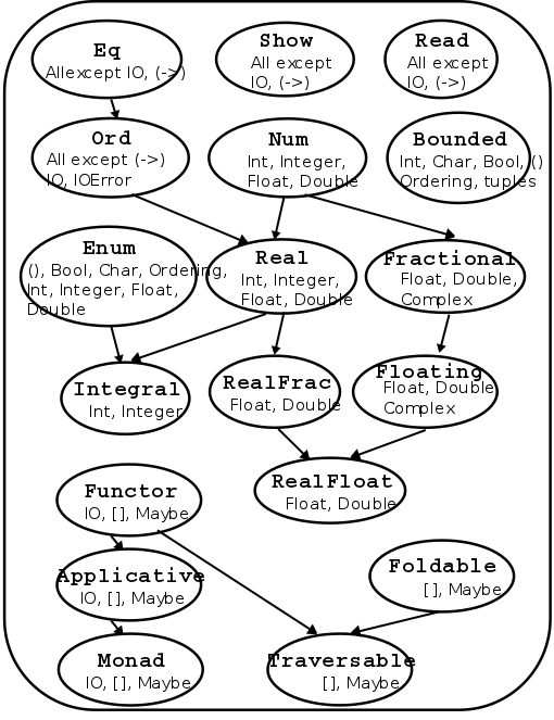
The classes are not all mutually exclusive. Ord supports < and >, but so does Real, because they’re numbers. Which do we pick; Ord or Real?
In reality, Real “extends” Ord, or is the ‘child’ of Ord. Real has all the functionality of Ord, and then some.
Here is a hierarchy of the classes:

Functions

Guarded equations

Haskell has if statements, but they can get very messy very quickly. You should never use them.
Instead, you can use guarded equations, which allow you to change the behaviour of a function based on a predicate (condition that returns true or false).

For example, let’s take the factorial recursive algorithm. It can do two things: return 1 when the input is 0 (base case), or multiply the input by factorial(input - 1) (recursive clause).
In Haskell, you can do this in two ways:

Pattern matching	Guarded equations
fact 0 = 1 fact n = n * fact (n - 1) {- Keep in mind that this only works for a .hs file, it will not work on the GHCi interface unless you use :{ and :} -}	fact n \| n == 0 = 1 \| n == 1 = 1 \| otherwise = n * fact (n - 1) {- In theory, you should be able to leave out the n == 1 bit, but GHCi didn't like it when I tried that. -}

Let’s take the guarded equation method and pick it apart to see how this works:

Steps	Value of n	Explanation
fact n \| n == 0 = 1 \| n == 1 = 1 \| otherwise = n * fact (n - 1)	2	Here, we start by inputting the value of ‘n’ into the factorial function.
fact n \| n == 0 = 1 \| n == 1 = 1 \| otherwise = n * fact (n - 1)	2	Now, we look at the first guarded equation predicate. If this is true, we do whatever is on the right of the equals sign next to it. If this is false, we move on to the next predicate.
fact n \| n == 0 = 1 \| n == 1 = 1 \| otherwise = n * fact (n - 1)	2	It’s false, so we look at the next predicate below it. The same rule applies here.
fact n \| n == 0 = 1 \| n == 1 = 1 \| otherwise = n * fact (n - 1)	2	It’s false, so we move on to the next predicate. The same rule applies here. ‘otherwise’ is like ‘else’ in Java or C, it’s used when all other predicates are false. It’s syntactic sugar for “True”.
fact n \| n == 0 = 1 \| n == 1 = 1 \| otherwise = n * fact (n - 1)	2	‘otherwise’ is always true, so we do what’s on the right of the equals sign here. This is the recursive clause, so we do the function again, but with n - 1.
fact n \| n == 0 = 1 \| n == 1 = 1 \| otherwise = n * fact (n - 1)	1	Here, we input the value of ‘n’ into the factorial function again.
fact n \| n == 0 = 1 \| n == 1 = 1 \| otherwise = n * fact (n - 1)	1	We check the first predicate. If it’s true, we do whatever is on the right. If not, move on to the next predicate.
fact n \| n == 0 = 1 \| n == 1 = 1 \| otherwise = n * fact (n - 1)	1	That was false, so we move on to the next predicate.
fact n \| n == 0 = 1 \| n == 1 = 1 \| otherwise = n * fact (n - 1)	1	That predicate was true, so we do what’s on the right of the equals sign next to it. It just says 1, so we return 1.

The order of the guards matter (just like if statements in Java), as the interpreter will go from top to bottom.

Using guarded equations, we can put error cases in our functions, like in this function that solves quadratic equations:

quadroots :: Float -> Float -> Float -> String
quadroots a b c | a == 0 = error "Not quadratic"
| b*b-4*a*c == 0 = "Root is " ++ show (-b/2*a)
| otherwise = "Upper Root is "
++ show ((-b + sqrt(abs(b*b-4*a*c)))/2*a))
++ "and Lower Root is "
++ show ((-b - sqrt(abs(b*b-4*a*c)))/2*a))

This is a little ugly, though... isn’t there some way we can locally define constants?

‘where’ vs ‘let’ and ‘in’

‘where’ allows you to locally define constants within the scope of your functions.
Using the quadratic example above, we can do:

quadroots :: Float -> Float -> Float -> String
quadroots a b c | a==0 = error "Not quadratic"
| discriminant==0 = "Root is " ++ show centre
| otherwise = "Upper Root is "
++ show (centre + offset)
++ " and Lower Root is "
++ show (centre - offset)
where discriminant = abs(b*b-4*a*c)
centre = -b/2*a
offset = sqrt(discriminant/2*a)

Now, the local variables ‘discriminant’, ‘centre’ and ‘offset’ are available within the scope of the function!
Doing this helps tidy up code and aid readability.
Make sure to indent the left of ‘where’ appropriately, or the Haskell interpreter will complain.

‘let’ and ‘in’ allows you to also define local variables inside a scope.
Example:

add x y = let z = x + y in
z

In this example, we have a function ‘add’ that takes in ‘x’ and ‘y’.
In that function, we let ‘z’ equal ‘x’ + ‘y’ within the scope of the next line.
In that next line, we’re not really doing much; we’re just returning z.
We can add more local variables using brackets, just make sure you use semi-colons:

quadadd a b c d =
let { e = a + b; f = c + d } in
e + f

This has exactly the same effect as this, where we nest ‘in’ clauses:

quadadd a b c d =
let e = a + b in
let f = c + d in
e + f

The difference between ‘let’ + ‘in’ and ‘where’ is that ‘let’ + ‘in’ is an expression; you can put it anywhere where an expression is expected. On the other hand, ‘where’ is syntactically bound to a function, meaning you can only use it in one place.

Pattern matching

You can define a function in several parts by using pattern matching.
Pattern matching allows you to define what the parameter should look like, and then act accordingly.
For example:

not :: Bool -> Bool
not False = True
not True = False

If the parameter is ‘False’, return ‘True’. If the parameter is ‘True’, return ‘False’.
Let’s try a more complex example:

nonzero :: Int -> Bool

nonzero 0 = False

nonzero _ = True

That underscore _ is a wildcard. Any value can go there, within reason. You use this when you don’t really care what’s there.
Again, the order of the pattern matches matter, just like guards.

Let’s try another:

(&&) :: Bool -> Bool -> Bool
True && b = b
False && _ = False

If I were to use the function like:

True && ((5 * 3 + 1) < (8 * 2 - 6))

The value of the expression on the right will be localised within the variable ‘b’ in the code above.

With structure patterns, you can apply pattern matching with structures, like lists or tuples.
For example, if you had:

foo (x,_) = x

This function foo, returns the first element of the input tuple: x.
The second element of the input tuple would be ignored, as there is a wildcard there.
Another example:

foo [5, a, 4] = a

As long as the first and third elements are ‘5’ and ‘4’, the result will be the second element.
This also works with nested tuples and nested lists.

With list patterns, you can use the ‘cons’ operator with pattern matching.
For example:

tail (x:xs) = xs

If you did tail [1,2,3], then the variable ‘x’ would be ‘1’ and ‘xs’ would be [2,3].
Basically, (x:xs) splits the list into its head and its tail. Sometimes, this makes implementing recursive algorithms easier. It also validates input to only lists with at least one element.
If (x:xs) = [1,2,3] then x = 1, xs = [2,3]
If (x:xs) = [4] then x = 4, xs = [ ]
You can go further and add more, like:

addFirstTwoFromList (x:y:xs) = x + y
oneElementOnly (x:[]) = True

With composite patterns, you can use all of the above together with multiple arguments.
Here is an example of that:

fetch :: Int -> [a] -> a
fetch _ [] = error "Empty List"
fetch 0 (x:_) = x
fetch n (_:xs) = fetch (n-1) xs

As you can see, pattern matching can be applied to any parameter, and can be used as extensively as you need, within reason.

String patterns are just normal patterns, but with strings.
Remember, they’re just lists of Chars. Therefore, list patterns can be used with strings.
For example, ( _ : ‘a’ : _ ) matches strings whose second character is ‘a’.
The pattern [] matches the empty string.

Lambda expressions

Lambda expressions are simple ways of creating quick functions without a name.
For example, you could create an add function and apply it like:

add :: Int -> Int -> Int
add x y = x + y

add 5 6

But did you know that you could also do:

(\x -> \y -> x + y) 5 6

(\x y -> x + y) 5 6

You don’t have to name it at all; you can just create it quick, use it, and never refer to it again.
This is particularly useful when using functions like ‘map’.

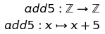
Operator sections

An operator section is an infix operator in prefix form:

(⊙), (x⊙), (⊙x)

Let’s say you wanted a function that just adds 5 to stuff.
You could write:

add5 :: Int -> Int
add5 x = x + 5

But why write that when you can write:

(+5)

This is because something like “5 + 4” can be written as “(+) 5 4”.
So you can cut that expression in half and get just the part where it adds 5: “(+5) 4” (because, remember, everything is curried in Haskell).
It works both sides, so (+5) and (5+) are the same.

List Comprehension and Recursion

List comprehension

You can generate a list, a bit like set comprehension.

[x^2 | x <- [1..5]]

Those two expressions yield the same thing, except one is set theory and one is Haskell.

Let’s pick it apart:

[x^2 | x <- [1..5]]
The blue part is what will be in each element of the list.
The red part are the conditions that each element must abide by.

You can even add more variables and conditions:

[(x,y) | x<- [1..5], y <- [6..10], x > y]

In general, list comprehensions look like this:

[exp | cond1, cond2, cond3, ..., condn]

Zips

There is a zip function, which lets you zip two lists together into tuples.
Example:

> zip ['a', 'b', 'c'] [1, 2, 3, 4]
[ ('a', 1), ('b', 2), ('c', 3) ]

STICKY FINGAAS!!!

This is pretty handy; you could use a list comprehension over the zipped list.
For example, you could pair up elements of a list:

pairs :: [a] -> [ (a,a) ]
pairs xs = zip xs (tail xs)

> pairs [1,2,3,4]
[(1,2),(2,3),(3,4)]

Then you could use a list comprehension to check if a list is sorted:

sorted :: Ord a => [a] -> Bool
sorted xs = and [ x≤y | (x,y) <- pairs xs ]

Recursion

Recursion is simple in Haskell.
Just refer to the same function again within the function body:

fac 0 = 1
fac n = n * fac (n-1)

If you need to recurse through a data structure, like a list, just do the following:

length :: [a] -> Int
length [] = 0
length (x:xs) = 1 + length xs

By doing this, ‘x’ is the first element of the list and ‘xs’ is the rest of the list.
You can also use wildcards:

drop 0 xs = xs
drop _ [] = []
drop n (_:xs) = drop (n-1) xs

You can also have mutual recursion, where two recursive functions recurse each other!

evens :: [a] -> [a]
evens [] = []
evens (x:xs) = x : odds xs

odds :: [a] -> [a]
odds [] = []
odds (x:xs) = evens xs

These are the 5 steps to not lose marks in the exam better recursion:

Step 1: Define the Type
Step 2: Enumerate the Cases
Step 3: Define the simple (base) cases
Step 4: Define the other (inductive) cases
Step 5: Generalise and Simplify

Tail recursion

Tail recursion is a special kind of recursion that calls itself at the end (the tail) of the function in which no computation is done after the return of recursive call.
In other words, the recursive calls do all the work, and at the end, the answer is just returned, as opposed to normal recursion, where a big computation is built up through recursive calls, then at the end, the whole thing is computed and returned.
Typically, tail recursion uses accumulators, whereas normal recursion does not.

Here are two kinds of factorial function, one with tail recursion and one without:

Tail recursion	No tail recursion
fac' :: Int -> Int -> Int fac' acc 0 = acc fac' acc n = fac' (n*acc) (n-1) fac' 1 5 -- Start fac' 5 4 fac' 20 3 fac' 60 2 fac' 120 1 fac' 120 0 120	fac :: Int -> Int fac 1 = 1 fac n = n * fac (n-1) fac 5 -- Start 5 * fac 4 5 * 4 * fac 3 5 * 4 * 3 * fac 2 5 * 4 * 3 * 2 * fac 1 5 * 4 * 3 * 2 * 1 120

In the tail recursion version, all of the work is done in the accumulator as each of the steps go by. Then, once the base case is reached, the answer is simply spat out.
In the non-tail recursion version, no work is done by the recursive steps; it’s just building up one big sum. Once the base case is reached, one huge computation is calculated and returned.

That’s the difference; tail recursion does stuff in steps, whereas normal recursion does it in one huge chunk at the end!

They still do the same thing, except tail recursion uses an accumulator.
Sometimes, the tail recursion way is easier to understand.

Because of the way Haskell works, these two methods work exactly the same way, even under the hood!
That’s because Haskell is lazy, and won’t calculate things unless it really has to.
So Haskell won’t calculate the value of the accumulator until the very end, which is what the non-tail recursion method does.

Higher Order Functions

A higher order function is a function that either takes in a function or returns a function.
The following are higher order functions:

func1 :: (a -> b) -> a

func2 :: a -> (b -> a)

Map, filter and fold

Why do we have higher order functions?
One of the reasons why is for the ‘map’ function.
The ‘map’ function allows you to apply a function to all elements of a functor.
For example, you could use ‘map’ to add 5 to all elements of a list:

map (\x -> x + 5) [1,2,3]

map (+5) [1,2,3]
-- result is [6,7,8]

Another example is ‘filter’, which allows you to filter out things from a list:

filter (\x -> x == 5) [1,2,3,4,5]

filter (==5) [1,2,3,4,5]
-- result is [5]

Another example is ‘fold’. There are two fold functions: ‘foldl’ and ‘foldr’.
‘foldl’ is left-associative, and ‘foldr’ is right-associative.
Here is an example that sums a list:

foldr (\x acc -> x + acc) 0 [1,2,3]

foldr (+) 0 [1,2,3]

The first argument is a lambda with an element and an accumulator, the second argument is the starting value of the accumulator and the third argument is the list to fold.
‘foldl’ works pretty much the same way as ‘foldr’, except for the different associativity, but there may be some efficiency gains. However, be wary of infinite lists with ‘foldl’!

Dollar operator

The operator $ takes in a function and an argument and applies the function to the argument.
Why not just run the function?
The reason why is $ associates to the right.
Here’s an example: let’s say you wanted to run the following:

sqrt 3^2 + 4^2

The answer you want is 5, but instead, you get 19. Why?
Haskell is left-associative, so it does sqrt 3^2 first, then adds it to 4^2.
To make it right, use this:

sqrt $ 3^2 + 4^2

The $ operator associates to the right, so 3^2 + 4^2 will be calculated first, then it’ll be square-rooted.

Function composition

Another operator is the function composition (dot) operator.
You can use it like maths, to join two functions together.
So instead of

odd x = not (even x)

Instead, you can write:

odd = not . even

That’s basically English!

Declaring Types

Declaring Types and Classes

‘type’

You can define type synonyms, so that you can call a data structure a name that makes more sense.
For example, we don’t say a character array (unless you’re working with C), we say ‘string’.
We don’t use [Char], we use String.
Here is how you can define your own synonyms:

type Pos = (Int, Int)

So now, instead of saying (Int, Int), you can say Pos instead.
If you want to parameterise the class you want, you can do that as well:

type Pair a b = (a,b)

So now, when you do function type declarations, you can feed in the class parameters of the synonym ‘Pair’, and those classes will be validated inside the tuple.
For example:

type Pair a b = (a, b)

f :: (Integral a, Integral b) => Pair a b -> Pair a b
f (x,y) = (x+1, y+1)

The function ‘f’ will only work if a pair of integers are inputted, because it takes in “Pair Integral Integral”.

Additionally, nesting types are allowed, but recursing them is not.

type Pos = (Int,Int)
type Translation = Pos -> Pos -- Niiicee!!

type Tree = (Int, [Tree]) -- Ohh noo!!

‘data’

If you want to define a completely new type, and not just a synonym, then you can use the ‘data’ keyword.
To instantiate a new type, you have to use it’s constructor.
Example:

data Pair = PairInt Int Int | PairString String String

To instantiate a new Pair, you need to use either the constructor PairInt, or PairString, then the values. This ensures type validation.
Here’s what’s allowed and not allowed with our example:

-- RIGHT

PairInt 5 6
PairString "filthy acts" "at a reasonable price"

-- W R O N G

PairInt "killer queen" "bites the dust"
PairString 4 4

You can have lots of constructors separated by bars |.

Like type synonyms, data types can have parameters too, like:

data Maybe a = Nothing | Just a

You can also do recursive types with ‘data’:

data BinaryTree a = Leaf a | Node a (BinaryTree a) (BinaryTree a)

Node 4 (Node 3 (Leaf 1) (Leaf 2)) Leaf 5 -- you could have this, for example

You can even do pattern matching:

getLeftBranch :: BinaryTree a -> BinaryTree a
getLeftBranch (Leaf a) = Leaf a
getLeftBranch (Node a x y) = x

‘newtype’

This is like a cross between ‘type’ and ‘data’. You can only have one constructor, and you can only provide one type after a constructor.
For example:

newtype Pair = Pair (Int, Int)

This means it’s more than just renaming something, because you still need the constructor, but it’s more restrictive than ‘data’ because you only have one constructor and one type.

‘class’

You know how each class has their own function that applies to every type that inherits that class?
For example:

the class Eq has ==
the class Ord has < and >
the class Num has + and -
the class Functor has ‘map’ (more on that later!)

Let’s make our own, using the ‘class’ keyword!
Example:

class Tree a where
flatten :: a b -> [b]

This is our ‘Tree’ class that represents trees. It has a method ‘flatten’, which flattens all of the values in the tree nodes.
The ‘a’ in ‘Tree a’ represents the data structure that inherits the ‘Tree’ class, for example ‘BinaryTree’.
The ‘b’ in ‘a b’ represents the type of the node values in the data type ‘a’.

So now, we have our class, like Eq or Ord.
But Eq and Ord have their own instances, for example all numbers inherit the class Eq or Ord. How do we create data structures that inherit our class Tree?

‘instance’

We can use the ‘instance’ keyword to pair our BinaryTree data type to our Tree class:

instance Tree BinaryTree where
flatten (Leaf v) = [v]
flatten (Node v x y) = [v] ++ flatten x ++ flatten y

In our instance block, we have to define the functions we’ve declared in the class block.
We need to define it in terms of BinaryTree, because that’s what we’re making an instance of.
So ‘class’ defines what Tree does generally with data type ‘a’, and ‘instance’ substitutes in ‘BinaryTree’ for ‘a’ and tells Haskell what to do if the program treats BinaryTree like a Tree.

If that doesn’t make any sense, then go ahead and try creating your own class with data types. You’ll learn much better by doing, not reading!

Trees

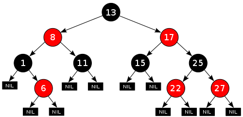
Red-Black Trees

Remember red-black trees from Algorithmics?

The root is black
All the leaves are black
If a node is red, it has black children
Every path from any node to a leaf contains the same number of black nodes

Here is an example of a balanced red-black tree:

How do we do this in Haskell?
Like this:

data RBTree a =
Leaf a
| RedNode a (RBTree a) (RBTree a)
| BlackNode a (RBTree a) (RBTree a)

We can also define a function called ‘blackH’ which finds the maximum number of black nodes from any path - from the root to the leaf.

blackH (Leaf _ ) = 0
blackH (RedNode _ l r) = maxlr

where maxlr = max (blackH l) (blackH r)
blackH (BlackNode _ l r) = 1 + maxlr
where maxlr = max (blackH l) (blackH r)

Abstract Syntax Trees

You can create a tree that represents syntax of an algebra.
For example, you could do arithmetic:

data Expr = Val Int | Add Expr Expr | Sub Expr Expr
eval :: Expr -> Int
eval (Val n) = n
eval (Add e1 e2) = eval e1 + eval e2
eval (Sub e1 e2) = eval e1 - eval e2

-- Example
eval (Add (Val 10) (Val 20)) -- Would return 30
eval (Sub (Val 20) (Val 5)) -- Would return 15

Even propositional logic:

-- Data type for propositional expression
data Prop = Const Bool
| Var Char
| Not Prop
| And Prop Prop
| Imply Prop Prop

-- Data type for a single pair of variable to value
type Subst = [ (Char, Bool) ]

-- Takes a var, a substitution pair and returns the value that the var is paired with
find :: Char -> Subst -> Bool
find k t = head [ v | (k',v) <- t, k == k' ]

-- Evaluates a propositional expression
eval :: Subst -> Prop -> Bool
eval s (Const b) = b
eval s (Var c) = find c s
eval s (Not p) = not $ eval s p
eval s (And p q) = eval s p && eval s q
eval s (Imply p q) = eval s p <= eval s q

-- Examples
eval [] (And (Const False) (Const True)) -- Would return False
eval [('a', True)] (Var 'a') -- Would return True

Functors

A functor is simply a class, like Ord or Num, that says “this can be mapped over”.
For example, a list is a type of functor, because you can use the “map” function on it.
The only function in this class is “fmap”. “map” is the same as “fmap”, except that it’s exclusively for lists.

Here is the class for Functor, as well as some instances:

class Functor f where
fmap :: (a -> b) -> f a -> f b

instance Functor [] where
fmap = map

instance Functor Maybe where
fmap _ Nothing = Nothing
fmap g (Just x) = Just (g x)

When you create an instance of Functor in some class you make, make sure it abides by the following laws:

Law 1:

fmap id = id

Law 2:

fmap (g.h) = fmap g . fmap h

Here is an illustration of fmap (+3) (Just 2)

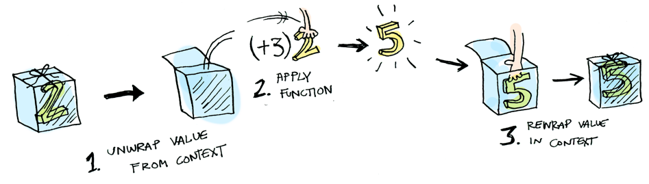
If you still don’t understand functors, I strongly suggest this article about Functors, Applicatives and Monads. It has really simple explanations and images to explain these complex ideas!

A tree is also a type of data structure. We could create a map function that works on trees, thereby making trees a functor!
We could have something like:

instance Functor BinaryTree where
fmap g (Leaf v) = Leaf (g v)
fmap g (Node v x y) = Node (g v) (fmap g x) (fmap g y)

Boom! Now we can use fmap on BinaryTrees if we wanted to, like:

fmap (\x -> x + 10) (Node 5 (Leaf 3) (Leaf 6))
-- this will return: Node 15 (Leaf 13) (Leaf 16))

Directions, trails and zippers

We can define the direction in which we can traverse through a tree, like this:

data Direction = L | R
type Directions = [ Direction ]

elemAt :: Directions -> Tree a -> a
elemAt _ (Leaf x) = x
elemAt (L:ds) (Node _ l _) = elemAt ds l
elemAt (R:ds) (Node _ _ r) = elemAt ds r
elemAt [] (Node x _ _) = x

-- Examples
elemAt [L] (Node 5 (Leaf 3) (Leaf 4)) -- returns 3
elemAt [R, L] (Node 5 (Leaf 6) (Node 2 (Leaf 8) (Leaf 9))) -- returns 8

How do we know how far we’ve gone?
We can build up a trail so we know the direction we’ve gone in:

type Trail = [Direction]

goLeft :: (Tree a, Trail) -> (Tree a, Trail)
goLeft (Node _ l _ , ts) = (l , L:ts)
goRight :: (Tree a, Trail) -> (Tree a, Trail)
goRight (Node _ _ r , ts) = (r , R:ts)

-- Examples
(goLeft . goRight) (a, []) -- for some tree 'a', this will return (b, [L, R]) where 'b' is the subtree if you go right, then left in 'a'

You can also make a function to follow a trail, if you like.
But what if you want to go back up? You don’t remember the parent when you go left or right.
You can make it so that Direction stores the parent as well:

data BinaryTree a = Leaf a | Node a (BinaryTree a) (BinaryTree a) deriving (Show)

data Direction a = L (BinaryTree a) | R (BinaryTree a) deriving (Show)
type Trail a = [ Direction a ]

parentInDirection (L p) = p
parentInDirection (R p) = p

goLeft :: (BinaryTree a, Trail a) -> (BinaryTree a, Trail a)
goLeft (Leaf x, ts) = (Leaf x, ts)
goLeft ( p@(Node _ l _) , ts) = (l, (L p):ts)

goRight :: (BinaryTree a, Trail a) -> (BinaryTree a, Trail a)
goRight (Leaf x, ts) = (Leaf x, ts)
goRight ( p@(Node _ _ r) , ts) = (r, (R p):ts)

goUp :: (BinaryTree a, Trail a) -> (BinaryTree a, Trail a)
goUp (tree, ts) = (parent, restOfList)
where
latestMove = head ts
restOfList = tail ts
parent = parentInDirection latestMove

-- Example
(goUp . goLeft) (tree, []) -- this will return (tree, []) because goLeft followed by goUp effectively does nothing, like taking a step forward then taking a step back

ZIPPER MAN!

This concept of pairing one piece of data with another in a list of pairs has a name in functional programming: it’s called a zipper type.

Graphs

Functional programming is crap for modelling graphs.
Usually, if you wanted to work with graphs in a functional programming paradigm, you’d use a hybrid language, like JavaScript or F#.
In Haskell, we’ll look at three ways to try and model graphs.

Indexed collections of Nodes, Edges

This is a nonstructural approach.
This is the easiest and most intuitive way to do things.
Basically, you have a function that takes in a node and returns a list of adjacent nodes, like so:

graph :: Int -> [ Int ]

Actually, the lovely developers over at Haskell HQ has already done this! In the Data.Graph package, they have:

type Table a = Array Vertex a
type Graph = Table [ Vertex ]

Where ‘Vertex’ is some ID of the node, like an Int or something.
They also provide functions for working with graphs, like searching, building, fetching, reversing etc.
This is alright, but you can’t weight the edges and the performance is slow.

Structured data type with cyclic dependencies

This has limitations for modifying the graphs.
It’s similar to the method from before, except we’re not using an array; we’re using a cyclic dependency.

What’s a cyclic dependency? Think of it like this:
What is the value of xs = 0 : xs?
It’s an infinite string of zeroes: [0,0,0,0,0,0,0,0,0...]
Next: what is the value of xs where xs = 0 : ys, ys = 1 : xs?
This one’s a bit more tricky, but it’s [0,1,0,1,0,1,0,1...]
So you see, we’re defining these lists in a “cyclic” manner, because they go back and forth, around and around, like a circle.

What if we applied a cyclic dependency to our graph structure?
First of all, to make it simpler, let’s assume that each node only has one edge.
Let’s create a data structure for this:

data Graph a = GNode a (Graph a)

Where:

GNode a (Graph a)
The value of the node
Adjacent node; the node that this node can go to

Now, we want a function that converts a table of nodes to a Graph structure:

mkGraph :: [ (a , Int) ] -> Graph a

Where our input table looks a little something like this:

ID	Value	Next node
1	London	3
2	Berlin	4
3	Rome	2
4	Morioh	1

The implementation can go a little something like this:

mkGraph :: [ (a, Int) ] -> Graph a
mkGraph table = table' !! 0
where table' =
map (\(x,n) -> GNode x (table'!!n) ) table

You can generalise this so that a node can have lots of outgoing edges:

data GGraph a = GGNode a [GGraph a]

mkGGraph :: [ (a, [Int]) ] -> GGraph a
mkGGraph table = table' !! 0
where table' =
map (\(x,ns) -> GGNode x (map (table'!!) ns ) table

With this method, you don’t need to name nodes and it’s fast to go from node to node. However, you can’t build this structure incrementally; you have to build it all at once.

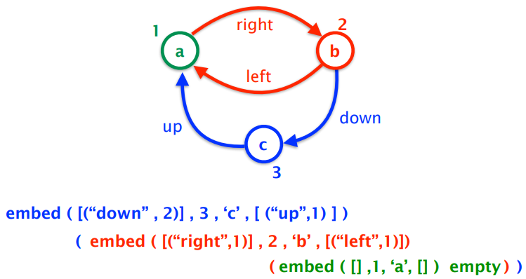
Inductive approach with graph constructors

This provides inductive structure and pattern matching.
This is the library Data.Graph.Inductive.Graph.
Here, each node has an Int ID, like last time.
The graph is built one node at a time, and all the nodes link together to form a graph, kind of like how you could use a : b : c to form a list [a,b,c].

There are two key things to building a graph using this approach:

empty :: Graph a b
embed :: Context a b -> Graph a b -> Graph a b

The ‘empty’ value is an empty graph with no nodes or edges.
The ‘embed’ function embeds a new node into an existing graph and returns the new graph.
So, what’s a context?
A context is a data structure that represents a node, on its own, outside a graph.
It stores the node ID, the node label, the outgoing edges and incoming edges.

type Adj b = [ (b,Node) ]
type Context a b = (Adj b , Node, a , Adj b)

Where Adj is:

type Adj b = [ (b,Node) ]
The label of the edge
The node on the end of this edge

And Context is:

type Context a b = (Adj b, Node, a, Adj b)
Incoming edges
Node ID of this node
Label of this node
Outgoing edges

An example of a graph with this is:

Of course, there are other ways to make this graph, which will all work if implemented.

Not only can you build up a graph node by node, you can decompose a graph node by node as well.
FGL provides a function ‘match’:

match :: Node -> Graph a b -> Decomp a b

Which takes in a node to remove, the graph itself, and returns the graph without the node.
Decomp is:

type Decomp a b = ( Maybe (Context a b), Graph a b )

Where:

the first element of the pair is either the removed node or nothing.
the second element of the pair is the graph without the node.

There’s also a function called matchAny:

matchAny :: Graph a b -> Decomp a b

If you don’t really care which node you take out; it’ll remove any.
With these, you can create a map function for your graph:

gmap :: (Context a b -> Context c b) -> Graph a b -> Graph c b
gmap f g

| isEmpty g = empty
| otherwise = embed (f c) (gmap f g')
where (c, g') = matchAny g

Evaluation Order and Laziness

Equational reasoning

Equational reasoning simply means proving things by following equations through.
For example, you could prove not (not False)) is False by simplifying it to not (True), then simplifying it further to False.

However, we’re going a little deeper by using proof by induction.
Proof by induction:

To prove P(n) for all n, we prove P(0) and we then prove for any k that P(k+1) holds under the assumption that P(k) holds.

Say we had the natural number data type, like this:

data Nat = Zero | Succ Nat

Where 0 is Zero, 1 is Succ Zero, 2 is Succ Succ Zero etc.
We also have an add function:

add :: Nat -> Nat -> Nat
add Zero m = m
add (Succ n) m = Succ (add n m)

How do we prove that ‘add’ is associative with proof by induction?
We need to prove it for a base case and for an inductive case.
We want to prove: add x (add y z) = add (add x y) z

Base Case	Inductive Case
add Zero (add y z) -- START add (add Zero y) z -- GOAL add Zero (add y z) = { defn of add } add y z = { defn of add 'backwards'} add (add Zero y) z	add (Succ x) (add y z) -- START add ( (add (Succ x) y) z ) -- GOAL add (Succ x) (add y z) = { defn of add } Succ (add x (add y z) ) = { inductive hypothesis } Succ (add (add x y) z) = { defn of add 'backwards'} add (Succ (add x y) z ) = { defn of add 'backwards'} add ( (add (Succ x) y) z )

You can even perform proofs on structures!
To see these proofs, look at the slides.

Redex

A redex, or “reducible expression”, is simply a part of an expression that you need to know before you compute the full expression.
For example, if you were to calculate the expression:

(1 + 5) * (6 - 3)

There are three redex’s inside this:

(1 + 5) * (6 - 3)

1 + 5
(1 + 5) *
6 - 3

Because Haskell is fully functional, expressions like “5 +” is actually a function, so to do, say, “5 + 6”, Haskell finds the function “5 +”, then uses that function on “6”.
Therefore, even in an expression like “5 + 6”, there is a redex “5 + 6” because Haskell needs to know that function before computing the rest of the expression.

Beta-reduction

Beta reduction is a process that converts a function call into an expression.
You’re familiar with lambda expression, right? You should be; I covered it a few sections ago.
If not, it goes like this: , where the first ‘x’ after the lambda is the parameter and everything after the dot is the function body. The syntax can vary, but that’s the gist of it.
You can call a lambda function like this: , which is .
If you wanted multiple parameters, you would do , which is (it’s similar to how Haskell curries everything).

When we converted to , we’ve done beta reduction.
More generally, if we had a function and an input , to beta reduce, just take the function body and replace all with .
Just like in our example, we took the function body and replaced all with .

Here’s a more complex example: how do we reduce...

...using beta reduction?
This is a big jump, but if we break this up and do this step-by-step, it’s not so bad.
First of all, let’s isolate the function body:

Now let’s split this up into its terms:

Our argument is . Which of those terms are ?
Just the one, right? So we replace that:

Now we work back into the function body...

... and we’re done.

Call-By-Name

Outermost reduction with no reduction under lambda is more commonly known as call-by-name reduction. This is used by Haskell.
In layman’s terms, this means that function calls are processed without processing or even looking at the arguments.

For example, let’s say we have an infinite list, and we want to get the first element of that infinite list:

take 1 [1, 2, 3, 4...]

Call-by-name doesn’t care about the infinite list; it won’t try to process it. Instead, it’ll just perform the function “take 1” and take 1 element off of that list. The result will simply be [1].
Because of this, Haskell can efficiently process information by lazy evaluation.

Haskell also uses something called graph reduction to perform lazy evaluation.
Remember in beta-reduction where an expression is repeated wherever the function parameter is?
With graph reduction, only one instance of the expression is stored and multiple pointers to that expression are used instead.
Therefore, any reductions performed on the single copy will permeate throughout all references of that expression.

You want an example of graph reduction? Alright: consider this Haskell line:

replicate 10 (6π^2)

With call-by-name, we don’t care what that argument is. We just create a list of 10 unevaluated expressions of . But since they’re all unevaluated, if we tried to display this list, wouldn’t we have to calculate 10 times for each element?
You are wrong! Remember, Haskell uses graph reduction. There is only one ; every element in that list is a pointer to that one . Therefore, we only need to calculate once, then all the pointers will update.

Call-By-Value

Innermost reduction with no reduction under lambda is more commonly known as call-by-value reduction. This is used by languages like C++, Java, Python etc.
In English, this means that arguments are processed before the function is called.

For example, let’s say we have an infinite list, and we want to get the first element of that infinite list:

take 1 [1, 2, 3, 4...]

Call-by-value will try and process that infinite list, and it’ll be there forever because there’s no end to it. Therefore, this function call will not end.

Modularity

Let’s just say we want a Haskell program that yields us a list of 300 1’s. Here’s two different possible solutions:

Solution A (the good one)	Solution B (the crap one)
ones = 1 : ones take 0 _ = [] take _ [] = [] take n (x:xs) = x : take (n-1) xs take 300 ones	replicate 0 _ = [] replicate n x = x : replicate (n-1) x replicate 300 1

Solution A splits the code into data (ones) and control (take).
Solution B blends the two together.

Solution A is better because it’s more modulated, therefore:

it’s easier to debug
parts of it are reusable
easier to read and understand
you split the problem up into subproblems, making it easier to program

The point is, Haskell allows modularity through laziness.
You can use this for other examples too, like creating a list of all prime numbers using the Sieve of Eratosthenes (data), then taking the first 100 primes (control).

Strict application

If you wanted to, you could scrap all of this and use strict application.
Basically, it tells Haskell to evaluate the expression on the right before applying the function. It’s used with the ‘$!’ operator.
It’s mainly used for space efficiency, and it allows for true tail recursion.
Example:

Step	Code
1	square $! (1 + 2)
2	square $! (3)
3	square 3
4	9

Interpreters and Closures

Part 1 - Substitutions

We’re going to write an interpreter in Haskell!
What language should we interpret?
How about lambda calculus? The rules are pretty simple there.

Lambda calculus

What is lambda calculus?
It’s a formal system to express functions.
There are only three rules: variables on their own, function application and function abstraction.
Here they are:

Rule	Description	Format	Example
Variable	It’s just a variable on it’s own.	Just some symbol on it’s own x	x y
Function abstraction	A function definition	A lambda character, followed by a variable name, followed by a full stop, followed by the function body which is another lambda expression λ(some variable).(some lambda expression) They can be curried to have more parameters λ(some variable).λ(anothervariable).λ(yet another variable) … .(some lambda expression) Instead of dots, you can use an arrow, if you wish	λx.x λx.λy.y λx.λx.x λx.λy.λz.y OR λx→x λx→λy→y λx→λx→x λx→λy→λz→y
Function application	A function being applied to some expression	It’s just an expression separated by an expression with a space (a lambda expression) (another lambda expression) It represents calling a function with some input	λx.x x λx.λy.y y x y λx.λy.y λy.λy.y

Despite how simple it is, it can encode a lot of information.
It can encode arithmetic, logic, structured data etc.

A variable x is bound in the term λx → e and the scope of the binding is the expression e.
A variable y is free in the term λx → y because it was initialised outside of the scope of this function abstraction.
A lambda expression with no free variables is called closed.

Beta reduction syntax

Remember beta reduction a few sections ago?
If not, scroll up and read it. It’s literally right above this section.

We’re going to express beta reduction like this:

(λx → e1) e2
will be rewritten as
e1 [ x := e2 ]
Read it like “In e1, replace all x with e2”.

Alpha conversion

We have

(λx → (λy → x)) y
which is basically
(λy → x) [ x := y ]
which becomes
(λy → y)

Everything seems fine and dandy.
But what if we have this:

λy → ((λx → (λy → x)) y)
it will become
λy → (λy → y)

Ah... that’s not exactly what we wanted. That y is now bound by the inner function, not the outer function like it’s supposed to.
If only we could rename the parameter of the inner function...
What? That’s already a thing?

Alpha conversion renames an inner function so that you don’t get variable capture, which is a phenomenon that occurs in substitution when a free variable becomes bound by the term you substitute it into.
So if we rename the inner y to z, we can have:

λy → ((λx → (λz → x)) y)
it will become
λy → (λz → y)

Everything is fixed thanks to alpha-conversion!

With all of these rules, you can now build your interpreter!
If you really want to know how, look at these slides.

Part 2 - Machines

Plot twist! Part 1 is a load of crap and you shouldn’t implement interpreters that way.
Well, you can, but it’s really inefficient.

Environments

We have this lambda expression:
(λx -> x) e
With normal beta reduction, this becomes just
e
But what if we were lazy and just said
x (but we know that e is substituted as x)
We’re not explicitly replacing anything, we’re just storing a record of the substitutions.
Therefore, we could look up stuff when we need it.

This is the concept of an environment.
An environment records bindings of variables to expressions, just like a mapping.

For example, if we had the expression
(λx -> e1) e2
... and we wanted to use beta reduction with environments, we could go about this like:

	Expression	Environment
Before beta reduction	(λx -> e1) e2	Nothing
After beta reduction	e1	x is mapped to e2

How do we write this in proper syntax?
We’ll write
e | E
to represent an expression e in the environment E.
So now, our beta reduction looks like:
(λx -> e1) e2 | E ⟼ e1 | E [ x := e2 ]
Where E [x := e2] means environment E updated with the new binding of x to the expression e2.

Note that e1 may now contain free occurrences of x.
That means we should have a rule like:
x | E ⟼ “lookup x in E” | E
... so that we can look up free occurrences of x when we get to them.

Frames

Another improvement to our interpreter is to make it so that it only focuses on the subterm that needs evaluating next.
Keep in mind that everything that follows is tailored to a call-by-value strategy.

Have a think about what we actually do when we look at an expression:

Expression	What do we do?
x	It’s just a variable. We can’t simplify this down any further, so just leave it. It’s terminated.
λx -> e	This is just a lambda term on it’s own. We can’t simplify this any further, so leave it. It’s terminated.
(λx -> e1) e2	This is an application, which can be reduced. First of all, we reduce e2, then we perform beta reduction.
e1 e2	We can simplify this, also. If we’re doing left-most, we simplify e1 then e2, and if we’re doing right-most, we simplify e2 and then e1. We will be doing left-most for now.

So there’s two possibilities of simplifying things down: either we have a lambda application, or a normal application with two expressions.

When we simplify the lambda application, we take out the e2 and leave the rest, leaving just
(λx -> e1) [-]
Where [-] is a hole or an empty void where we took out e2 and can plug in other expressions.
Once we’ve simplified e2, we plug it back in and we perform beta reduction.

When we simplify the application, we take out e1, leaving just
[-] e2
Once we’ve simplified e1, we plug it back in and take out e2, leaving:
e1 [-]
Once we’ve simplified e2, we plug that back in and we can continue.

All of these expressions with [-] in them are called frames.
They’re sort of like a “snapshot” of what we haven’t evaluated yet as we venture deeper into the lambda expression.
Think of it like a Java call stack, how ‘frames’ are stacked when you call lots of methods.
A stack of frames is called a continuation.
Just for reference’s sake, a value is a terminated expression; one that cannot simplify anymore.

Continuations

Now that we have continuations, let’s rewrite our reductions as follows:
e | E | K ⟼ e’ | E’ | K’
Where K is our continuation.

When do we push a new frame onto the stack?
We push when we have an unevaluated expression that we want to simplify.
e1 e2 | E | K ⟼ e1 | E | ([-] e2) :: K

When do we pop a new frame off the stack?
If our focussed expression is terminated (which will be represented with a V), there’s three possibilities:
K is empty

We’re finished; the evaluation has terminated

K has [-] e2 at the top

We now need to take out e2 and put back e1 (now called V because we should have simplified it), by popping the e2 frame and pushing a new frame with V on it:
V | E | [-] e2 :: K ⟼ e2 | E | V [-] :: K

K has (λx -> e1) [-] at the top

We need to perform beta reduction:
V | E | (λ x -> e) [-] :: K ⟼ e | E [x := V] | K

CEK-machines

Let’s combine these three ideas into one set of rules.
This is called a CEK-Machine, and it stands for:

Control
Environment
Kontinuation

Each of these make up the syntax we’ve been using all this time:

e | E | Kg

Here’s the rules, in all their glory:

#	C	E	K	C	E	K
1	x	E	K	“lookup x in E”	E	K
2	e1 e2	E	K	e1	E	[-] e2 :: K
3	V	E	[-] e :: K	e	E	V [-] :: K
4	V	E	(λx -> e) [-] :: K	e	E [x := V]	k

R1: x | E | K ⟼ “lookup x in E” | E | K

R2: e1 e2 | E | K ⟼ e1 | E | [-] e2 :: K

R3: V | E | [-] e :: K ⟼ e | E | V [-] :: K

R4: V | E | (λx -> e) [-] :: K ⟼ e | E [x := V] | K

Rule #	Explanation
1	If we see a single variable on it’s own, look it up in the environment and replace it with that corresponding expression.
2	If we see an application, take out the left expression for simplifying and put the right expression onto the stack.
3	If we have a fully simplified expression and there’s an application on the stack that has a left-side missing, put the left side back and take out the right-side for simplifying.
4	If we have a fully simplified expression and there’s a lambda application on the stack that has a right-side missing, perform beta reduction on our terminated value and that function application.

But not too much glory! There’s a problem.

Closures

What’s the problem?
Have a look at this expression:
(λz -> λx -> (λy -> y z x y) (λx -> z x)) e1 e2
This looks daunting at first, but let me split this up for you:
(λz -> λx -> (λy -> y z x) (λx -> z x)) e1 e2
Remember that z is e1 and x is e2.
Now, I want you to focus on this part here:
λy -> y z x
The y here is bound to the yellow function above, so:
(λx -> z x) z x
Now z is being substituted into this function as x, so now x is being rebound to the value of z, which is e1.
But that means our interpreter will change the x on the right of the expression into e1, when it should be e2.

When a function is used as a value, we need to keep track of the bindings of its free variables at the point of use.
We need to think of a function as a closed entity.
How do we do this?
We use closures!
A closure is a pairing of a function to the bindings in the current environment.
The syntax is: cl(λx -> e, E)
We pass these around instead of values.
Think of a closure like local scoped variables in a method in Java.

Here’s the new grammar we’re using:
W ::= cl(λx -> e, E)
F ::= W [-] | [-] e E
K ::= [] | F :: K
E ::= ∅ | E [x := W]
W represents a closure or a terminated value.
F is a frame
K is a continuation
E is an environment

Here’s the rules, but rewritten with closures:

#	C	E	K	C	E	K
1	x	E1	K	λx -> e	E2	K
2	e1 e2	E	K	e1	E	[-] e2 E :: K
3	λx -> e	E	K	cl(λx -> e, E)	E	K
4	W	E1	[-] e E2 :: K	e	E2	W [-] :: K
5	W	E1	cl(λx -> e, E2) [-] :: K	e	E2 [x := W]	K

R1: x | E1 | K ⟼ λx -> e | E2 | K where lookup x in E1 is cl(λx -> e, E2)

R2: e1 e2 | E | K ⟼ e1 | E | [-] e2 E :: K

R3: λx -> e | E | K ⟼ cl(λx -> e, E) | E | K

R4: W | E1 | [-] e E2 :: K ⟼ e | E2 | W [-] :: K

R5: W | E1 | cl(λx -> e, E2) [-] :: K ⟼ e | E2 [x := W] | K

Rule #	Explanation
1	A simple variable look-up, this time with closures. I’m not sure why the slides made it so complicated; it’s just a look-up as far as I can see.
2	If there is an application, pluck out the left-side and put the rest on the continuation stack along with a copy of the current environment.
3	If there is a function, wrap it in a closure along with a copy of the current environment.
4	If we have a terminated value and a right-side only application is on top of the stack, then take the right-side to simplify and put the left-side (our terminated value) back into the stack.
5	If we have a terminated value and a closure on the stack, then pop the closure off the stack, perform beta reduction with the closure function and the terminated value and add the new pairing to the environment.

Example sequence

In case you forgot, this is supposed to interpret lambda expressions.
Let’s watch this evaluate the term:
(λx → λy → x) e1 e2
Given that e1 and e2 are terminated values:

Step #	Rule # used	C	E	K	Explanation
1	N/A	(λx → λy → x) e1 e2	∅	[]	Nothing has been done yet; this is like our “initial state”.
2	R2	(λx → λy → x) e1	∅	([-] e2 ∅) :: []	We have an application, so R2 is applied. The left side of the application is plucked and stored in control, and a new frame is created and pushed, which stores the other side along with a copy of the environment at the time of creation.
3	R2	(λx → λy → x)	∅	([-] e1 ∅) :: ([-] e2 ∅) :: []	There is another application, so R2 is used again. Like with the previous step, the left-hand side is stored and the right-hand side is pushed as a frame, with a copy of the environment with it.
4	R3	cl(λx → λy → x, ∅)	∅	([-] e1 ∅) :: ([-] e2 ∅) :: []	A raw function is found! We apply R3. We create and store a closure of this function with the current environment.
5	R4	e1	∅	cl(λx → λy → x, ∅) [-] :: ([-] e2 ∅) :: []	We have a closure, and an application is on the stack. We use R4. This is just like the rule before closures, but this time it’s with closures; we put the left expression back and we now take out the right expression.
6	R5	λy → x	[x := e1]	([-] e2 ∅) :: []	We have a terminated value and a closure on the stack, so we use R5. We take out the environment in the frame and use that (which was nothing to begin with), then we add a new pairing: the parameter of the function in the closure to the expression in the control section. The expression in the function of the closure goes into our control section.
7	R3	cl(λy → x, [x := e1])	[x := e1]	([-] e2 ∅) :: []	We’ve found another raw function, so yet again, we put a closure around it and add a copy of the current environment to it.
8	R4	e2	∅	cl(λy → x, [x := e1]) [-] :: []	We’ve got a closure and another application on the stack, so we use R4. Simply, we put the left-side expression back and take out the right-side expression to simplify.
9	R5	x	[x := e1, y := e2]	[]	We have a terminating value and a closure on the stack, so we use R5. Again, the environment in the closure is used and we add an extra pairing of the closure function’s parameter to the expression in the control section. The body of the closure function is now in the new control section.
10	R1	e1	[x := e1, y := e2]	[]	We have a single value we need to convert, so we use R1, which looks up the value of x and replaces it with what it finds.
DONE

We’re finished; the expression simplifies down to just e1!

Functional I/O and Monads

I/O in Haskell

IO a

Pure function: a function whose output solely depends on the input. Nothing else affects the output.
This is not true with Java methods, because the state of the object also affects the output. This is called a side-effect.

A function with a side-effect in Haskell is a little hacky. Basically, we input a state along with the input, and we get a state out along with the output:

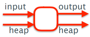
Let’s just say we had a type World that represents the system state.
We could define a transformation:
type IO = World -> World
We need an output too, so we should instead put:
type IO a = World -> (a, World)
Our function also needs to take arguments, so we can do:
Char -> IO a
Which would be the same as:
Char -> World -> (a, World)

So, what can you do with the World? Stop time?
No. It actually doesn’t exist.
But IO does.
So when you have a function like Char -> IO Int, this actually means this:

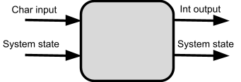
... and the Int you get out is determined by the Char input and the system state.

The difference between Int and IO Int is that:

Int is just a regular type that can store an integer
IO Int is a function that takes in a system state and returns an integer value and the modified system state

Actions

These are all actions:

IO Char
IO Float
IO ()
IO a

An action is an expression of type IO a.

There are three basic actions:

getChar :: IO Char (read a single character from stdin)
putChar :: Char -> IO () (takes a char and returns an action that writes that char to the standard output)
return :: a -> IO a (casts a pure expression into an expression with IO)

When we see an action of type IO (), it doesn’t return anything; its only purpose is to change the state in some way.

Do notation

How do we sequence actions, for example how do we call getChar 3 times in a row to read a string of length 3?
We can use do notation!
‘do’ notation looks like this:

do p1 <- act1
p2 <- act2

pn <- actn
actfinal

The actions are listed from act1 to actn, and any result is pattern matched and bound to p1 to pn.
The final action actfinal must not be bound and is typically a ‘return’ action.
Each action must be column aligned.
If an action doesn’t return anything, then you don’t need the “p <-” bit.
The type of the overall expression is the type of the final action.

This is an example of an action that reads three characters, and returns the first and third characters:

firstThird :: IO (Char,Char)
firstThird = do x <- getChar
getChar
y <- getChar
return (x,y)

This is an example of an action that writes a string to standard output:

putStr :: String → IO ()
putStr [] = return ()
putStr (x:xs) = do putChar x

putStr xs

This is an example of an action that writes a string to the standard output with a new line:

putStrLn :: String → IO ()
putStrLn xs = do putStr xs

putChar '\n'

This is an example of an action reading a line from standard input:

getLine :: IO String
getLine = do x <- getChar

if x == '\n' then

return []

else

xs <- getLine

return (x:xs)

The one above might take a bit of explaining:

The ‘if, then, else’ section is all one expression with type IO String and is thus an action.
The reason why we do a second ‘do’ at the end is because ‘else’ only expects one action after itself, and by using ‘do’ we encapsulate those two lines into one action.

Main Function, File Handling, Random Numbers

Did you know there’s a main function in Haskell?
It’s of the type IO ()

Haskell also provides basic actions for reading and writing files:

type FilePath = String
readFile :: FilePath -> IO String
writeFile :: FilePath -> String -> IO ()
appendFile :: FilePath -> String -> IO ()

As you would expect, reading files are done lazily.

The System.IO module introduces the IO type and the Handle type, so you can choose whether you want to read/write from stdin, stdout, stderr or a file.

You can also have random actions, from the System.Random module.
You can get a random number with:
randomIO : IO a
You can get a random number in a range with:
randomRIO :: (a, a) -> IO a

Applicatives

A quick refresher on functors: they’re classes that can be mapped over with fmap. Lists, Justs, Trees, they’re all functors.

Applicative is a class, like Functor. In fact, it’s the next step up from functors.
With applicatives, the function is now wrapped in a context!
The class looks like this:

class Functor f => Applicative f where
pure :: a -> f a
(<*>) :: f (a -> b) -> f a -> f b

The pure function takes any pure value and adds a context to it. Nothing is changed.
For example:

pure x = [x] (for lists)
pure x = Leaf x (for trees)
pure x = Just x (for maybes)
pure x = return x (for IO)

The <*> operator unpacks the function from the context and the argument, applies the function to the argument, and then packs the result back into a context and returns it.
So applicatives are just functors, but the function is in a context as well.
Here’s an illustration of Just (+3) <*> Just 2

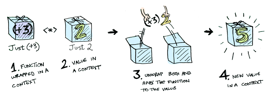
With this, we can create maps that handles multiple inputs!
For example:

pure (\x y -> x + y) <*> [1, 2, 3] <*> [10, 20, 30]

So, what does this actually simplify to?
You know that Haskell is left-associative, so the order goes like this:
pure (\x y -> x + y) <*> [1, 2, 3] <*> [10, 20, 30]
Where red is first and blue is second.
pure takes the input and adds a context to it, so it becomes
[\x y -> x + y] <*> [1, 2, 3] <*> [10, 20, 30]
Next, the red expression is simplified by unpacking the function and the argument and applying them.
However, notice that the function requires two parameters, but we’re only giving it one in this red expression. What happens when you give a function too little parameters? It returns a partially applied function!
So for each number (1, 2 and 3), that lambda on the left will not return a number; it’ll return a partially applied function for each, so the result will be:
[(\y -> 1 + y), (\y -> 2 + y), (\y -> 3 + y)]
Making our total expression:
[(\y -> 1 + y), (\y -> 2 + y), (\y -> 3 + y)] <*> [10, 20, 30]
Now we just have to simplify the blue bit. We’re comfortable with one function being wrapped in a list, but what about multiple?
What the list applicative does in this case is it unpacks all the functions, and it applies the first with all the argument values, the second with all the argument values etc. then it unions all those results into one big list.
So the result of this would be:
[11, 21, 31, 12, 22, 32, 13, 23, 33]
Which is our final answer.

Did you know that IO is also an applicative?
pure in terms of IO is the same as return.
<*> in terms of IO is the following:

(<*>) :: IO (a -> b) -> IO a -> IO b

mg <*> mx = do g <- mg

x <- mx

return (g x)

In English, <*> takes two actions as input:

An action that returns a function from a to b
An action that returns a value a

The operator unpacks the function and the value by performing the actions in a ‘do’ block. It then runs the function on the value and returns it out of the ‘do’ block.
Because return is the same as pure, return (g x) will return an action, or an IO b expression, because return and pure packs pure values into contexts (in this case, IO).

How is this useful?
We can use this to make a function
getChars :: Int -> IO String
... that reads the given number of Chars from stdin.

getChars :: Int -> IO String
getChars 0 = return ""
getChars n = pure (:) <*> getChar <*> getChars (n - 1)

We use : to stick all the characters together into a string, and we wrap it into an IO using pure (:).
Sure, we could also do

getChars :: Int -> String
getChars 0 = ""
getChars n = getChar : getChars(n - 1)

But that doesn’t give us an action. We can use the one that uses applicatives in a ‘do’ block, like this:

do
str <- getChars 5
return str

If you can’t be bothered to write pure for the first argument all the time, use <$>:

pure a <*> f b
is the same as
a <$> f b

Lastly, like with functors, there are applicative laws that you need to uphold when implementing them:
Law 1: Identity

pure id <*> x = x

Law 2: Homomorphism

pure (g x) = pure g <*> pure x

Law 3 (symmetry):

x <*> pure y = pure (\g -> g y) <*> x

Law 4 (transitivity):

x <*> (y <*> z) = (pure (.) <*> x <*> y) <*> z

If you still don’t understand applicatives, I strongly suggest this article.

Why are functors a superclass of applicatives?
If a class C is an applicative, then that means it has an implementation for the functions pure and <*>.
fmap can be defined using only pure and <*>:

fmap f x == pure f <*> x

Therefore class C can be a functor.

Monads

Monads take it a step even further:

class Applicative m => Monad m where
return :: a -> m a
(>>=) :: m a -> (a -> m b) -> m b
return = pure

So what does this actually mean?
Don’t worry too much about return; that’s just the same as pure.
The real defining feature of monads is the >>= operator (called ‘bind’).
The >>= operator takes a wrapped value and a function that returns a wrapped value, and applies the wrapped value to the function and returns another wrapped value.

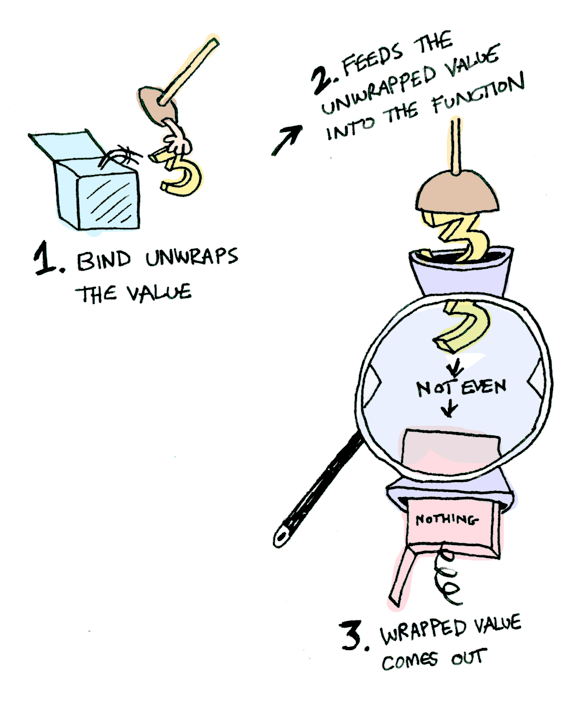
Don’t forget, like with functors and applicatives, there are monad laws too.
Law 1: Composition / Left Identity

return x >>= f = f x

Law 2: Identity / Right Identity

mx >>= return = mx

Law 3: Associativity

(mx >>= f) >>= g = mx >>= (\x -> (f x >>= g))

Why are applicatives a superclass of monads?
If a class C is a monad, then that means it has an implementation for the functions return and >>=.
pure and <*> can be defined using only return and >>=:

pure = return
f <*> x = f >>= \g ->

x >>= \y ->
return (g y)

Therefore class C can be an applicative.

That sounds so pointless; how could we ever use monads?
Monads are mainly used to abstract away boilerplate code, so that we can turn a complicated sequence into a succinct pipeline.
When you ask a computer to calculate the next three possible moves, would you write code along the lines of “Find the positions in the next move, but don’t go off the board or walk into any other pieces! Then, go through each of those new positions and find the next move of all of those, also making sure you don’t go off the board or walk into any other pieces! Then, go through each of those new positions and find the next move, and also make sure you don’t go off the board or walk into any other pieces etc.”
Look how long and tedious that is when all you needed was “Find the positions in the next three moves”. That’s the sort of thing that monads solve.
Remember, monads are just a design pattern. There’s nothing new; it’s just a different, more clean way of doing things.
Here’s examples of uses of monads: error handling, chaining and non-determinism.

Use of monads: Error handling

We have this data type:

data Expr = Val Int | Div Expr Expr

How do we evaluate it? Like this?

eval :: Expr -> Int

eval (Val n) = n

eval (Div x y) = eval x `div` eval y

What if we divide by 0? It’ll stop working.
How do we handle the case where we divide by 0?
We could return Maybe Int instead of Int, so we could return Nothing if we divide by 0.
Did you know that Maybe is a monad?
Maybes handle monads like this:

Just x >>= f	Nothing >>= f
Just (f x)	Nothing

So if nothing is passed in, nothing comes out, but if a Just is passed in, the function applies normally and another Just comes out.

Rewriting this with monads, we can do:

eval :: Expr -> Maybe Int
eval (Val n) = Just n
eval (Div x y) = eval x >>= \n ->
eval y >>= \m ->
safediv n m

safediv :: Int -> Int -> Maybe Int
safediv _ 0 = Nothing
safediv n m = Just (n `div` m)

So what’s actually going on here?
safediv is pretty easy; we’re dividing the numbers in a Just if the second number is not zero. If the second number is zero, we return nothing.
eval uses lambdas as functions, and uses safediv at the end to return another wrapped value.
This is good because if any ‘layer’ of those lambdas returns Nothing, then everything after it will be Nothing as well. This error handling is woven into monads, so we can abstract away that stuff out of our eval function.
We can actually rewrite eval to make it easier to read:

eval :: Expr -> Maybe Int
eval (Val n) = Just n
eval (Div x y) = do

n <- eval x
m <- eval y
safediv n m

Look familiar? This is the same ‘do’ notation that we used for IO.
This is because ‘do’ notation is actually syntactic sugar for that lambda stuff we did above.
If we used ‘do’ notation for IO, does that mean IO is a monad?
Yes. IO is a monad.

Use of monads: Chaining

You can also chain functions together with monads, like this:

Just 10 >>= (\x -> Just (x + 10)) >>= (\x -> Just (x * 2))

Let’s go over this bit-by-bit.
Remember, Haskell is left-associative so the expression is parsed like this:
Just 10 >>= (\x -> Just (x + 10)) >>= (\x -> Just (x * 2))

Where red is parsed first and blue is parsed second.
The bind unwraps the first argument, Just 10 to 10, and passes it through the given function, \x -> Just (x + 10). This results in:
Just 20
So now our expression is:
Just 20 >>= (\x -> Just (x * 2))
Again, we unpack Just 20 to 20. Then we pass it into the function, leaving us with:
40
This is our final answer! The functions x + 10 and x * 2 are chained together with bind, so the operation here is practically just 2(x + 10).

Use of monads: Non-determinism

What about lists? They’re monads too, you know.
How do lists handle bind? They do it like this:

xs >>= f = [ y | x <- xs, y <- f x ]

English, please:
This means the function is performed on each element of the list, and all of those results are collected or “unioned” into one big list.
For example, the expression:

[3, 4, 5] >>= \x -> [x, -x]

... will evaluate to:

[3, -3, 4, -4, 5, -5]

This is great because it allows us to do non-deterministic computations with very little code!

If you read the slides (or turned up to the lectures), you’ll remember the Knight’s Tour example.
Basically, we have a knight on a chessboard and we want to know the possible places it can move.
If you’ve never played chess before (play it, it’s hype) a knight can move one space left, up, down or right, then another two spaces in a perpendicular direction. For example, a knight could move one space up, then two spaces right.
Here, we’ll model it in Haskell:

type KnightPos = (Int,Int)

moveKnight :: KnightPos -> [ KnightPos ]

moveKnight (c,r) = filter onBoard

[ (c+2,r-1), (c+2,r+1), (c-2,r-1), (c-2,r+1),

(c+1,r-2), (c+1,r+2), (c-1,r-2), (c-1,r+2) ]

where onBoard (c,r) = c `elem` [1..8] && r `elem` [1..8]

In this code, the moveKnight method takes in a position and returns the possible positions of the next move. That’s great, but what if we want to know the possible positions of the next 3 moves?
Monads!

in3moves :: KnightPos -> [ KnightPos ]

in3moves start = return start >>= moveKnight >>= moveKnight >>= moveKnight

Let’s go over this...
Haskell is left-associative:
return start >>= moveKnight >>= moveKnight >>= moveKnight
The return function is just like pure; it wraps start into a list, the monad we’re working with.
[start] >>= moveKnight >>= moveKnight >>= moveKnight

The expression [start] >>= moveKnight will unpack [start] to get just start, then it will put it into moveKnight and that function will return a list of all the possible positions to move to from start within one turn.
[all possible moves in one turn]
This makes our expression:
[all possible moves in one turn] >>= moveKnight >>= moveKnight
Remember how lists work with monads? The bind operator runs the function on all of the elements of the list, then collects them all together into one big list.
So now, in the blue expression, moveKnight is being called on all elements of the [all possible moves in one turn] list. That means all the results we’ll get will be all the possible moves in two turns!
[all possible moves in two turns]
So our expression will become:
[all possible moves in two turns] >>= moveKnight
Like before, moveKnight is being called on all elements of [all possible moves in two turns], so all the results will be the possible moves in three turns.
[all possible moves in three turns]
Now we’re done! As you can see, if we can make a move in one turn, we can chain these together with bind and see where we’ll be in three turns by using list monads. Since lists can process things in a non-deterministic fashion, we can calculate different possible “paths”.
If you wanted to, you could see how many moves you could make in n turns just by repeating the bind call n times.

Remember, if you ever get confused about functors, applicatives and monads, just remember this picture:

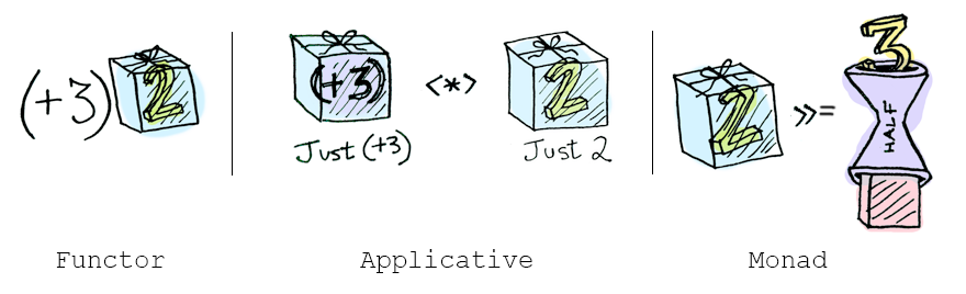
We’re not done with monads just yet. Sorry!
There’s two more functions: mapM and filterM.

mapM

The mapM function goes like this:

mapM :: Monad m => (a -> m b) -> [a] -> m [b]

mapM f [] = return []

mapM f (x:xs) = do y <- f x

ys <- mapM f xs

return (y:ys)

So what does this mean?
You pass in a function that takes pure values and outputs wrapped values:

... and you also pass in a list of pure values:

[ x1, x2, x3, x4, ..., xn ]

mapM will then do the following:

do
y1 <- f x1
y2 <- f x2
y3 <- f x3
.
.
.
yn <- f xn
return (y1 : y2 : y3 : ... : yn : [])

Basically, mapM is like normal map but with the benefit of monads (error handling, non-determinism etc.)

So, for example, if we did:

mapM (\x -> [x,-x]) [1,2,3]

We will get the result:

[[1,2,3],[1,2,-3],[1,-2,3],[1,-2,-3],[-1,2,3],[-1,2,-3],[-1,-2,3],[-1,-2,-3]]

Because that map is pretty much doing the same as:

x1 <- (\x -> [x,-x]) 1

x2 <- (\x -> [x,-x]) 2

x3 <- (\x -> [x,-x]) 3

return (x1 : x2 : x3 : [])

Still don’t get what this is saying? Don’t worry; let’s go through this.
I’ll use a table and steps to illustrate this properly:

Step #

Code

Values

Explanation

x1 <- (\x -> [x,-x]) 1

x2 <- (\x -> [x,-x]) 2

x3 <- (\x -> [x,-x]) 3

return (x1 : x2 : x3 : [])

x1 = N/A

x2 = N/A

x3 = N/A

We’ve just entered the ‘do’ block.

In the ‘Code’ column, the red highlighted bit shows the lines where the computation has already processed.

x1 <- [1, -1]

x2 <- [2, -2]

x3 <- [3, -3]

return (x1 : x2 : x3 : [])

x1 = N/A

x2 = N/A

x3 = N/A

Just to make things a bit easier for us, let’s simplify those lambda calls on the right. It’s easy to see what they return, and it’ll just complicate things if we leave them. It doesn’t change anything.

Normally, GHCI will lazily evaluate them, but just for the example’s sake, we’ve simplified those now.

x1 <- [1, -1]

x2 <- [2, -2]

x3 <- [3, -3]

return (x1 : x2 : x3 : [])

x1 = 1

x2 = N/A

x3 = N/A

Now, we’re looking at the first line.

Remember how list monads work? The bind operator runs the function on all the values within the list, so the function will run twice here: one with 1 as the input and one with -1 as the input.

But where’s the “function” here? We’re in a do block. Remember, do is syntactic sugar. If you look at this expressed with bind operators, you’ll see that our “function” is just the rest of the do block, the bits that aren’t highlighted in red.

So now, x1 is 1.

x1 <- [1, -1]

x2 <- [2, -2]

x3 <- [3, -3]

return (x1 : x2 : x3 : [])

x1 = 1

x2 = 2

x3 = N/A

Again, the same thing applies and the “function” here will be run twice: one with 2 and one with -2.

x1 <- [1, -1]

x2 <- [2, -2]

x3 <- [3, -3]

return (x1 : x2 : x3 : [])

x1 = 1

x2 = 2

x3 = 3

Yet again, the function will be called twice and x3 will be 3 and will soon be -3.

x1 <- [1, -1]

x2 <- [2, -2]

x3 <- [3, -3]

return (x1 : x2 : x3 : [])

x1 = 1

x2 = 2

x3 = 3

[1, 2, 3]

Now we’re at the return. Because we’re using the list monad, return will bunch these values all into a list, so it’ll return [1, 2, 3].

x1 <- [1, -1]

x2 <- [2, -2]

x3 <- [3, -3]

return (x1 : x2 : x3 : [])

x1 = 1

x2 = 2

x3 = -3

We’ve reached return; it’s all over, right? Hold it! Remember how the functions are repeated for each value in the list? Now, the computation falls back to x3. The function is called again and x3 becomes -3.

x1 <- [1, -1]

x2 <- [2, -2]

x3 <- [3, -3]

return (x1 : x2 : x3 : [])

x1 = 1

x2 = 2

x3 = -3

[1, 2, -3]

We now get [1, 2, -3] since x3 has a new value.

x1 <- [1, -1]

x2 <- [2, -2]

x3 <- [3, -3]

return (x1 : x2 : x3 : [])

x1 = 1

x2 = -2

x3 = N/A

x3 is done for this branch, but now we go further back and x2 becomes -2.

x1 <- [1, -1]

x2 <- [2, -2]

x3 <- [3, -3]

return (x1 : x2 : x3 : [])

x1 = 1

x2 = -2

x3 = 3

Now we’re going back into the x3 bit and x3 is going to become 3 and -3, except this time, x2 is -2.

x1 <- [1, -1]

x2 <- [2, -2]

x3 <- [3, -3]

return (x1 : x2 : x3 : [])

x1 = 1

x2 = -2

x3 = 3

[1, -2, 3]

We’ve reached return again, and now we’ve got [1, -2, 3].

Hopefully, you get the picture; all the combinations will be reached. I’m going to stop now, because this could go on for a while.

fitlerM

The filterM function goes like this:

filterM :: Monad m => (a -> m Bool) -> [a] -> m [a]
filterM p [] = return []
filterM p (x:xs) = do b <- p x
ys <- filterM p xs
return (if b then x:ys else ys)

What does this mean?
You pass in a function that takes pure values and outputs wrapped booleans:

... and you also pass in a list of pure values:

[ x1, x2, x3, x4, ..., xn ]

filterM will then do the following:

y1 <- p x1

y2 <- p x2

y3 <- p x3

yn <- p xn

return [ x1 if y1 is true (note: not actual Haskell!)

x2 if y2 is true

x3 if y3 is true

xn if yn is true ]

Basically, filterM is just like filter, except with the benefits of monads (error handling, non-determinism etc.)
It’s similar to mapM, except instead of mapping to another value, it uses a predicate and decides whether or not to include a value in a list depending on that predicate.
With it, you can make a function that gives you the powerset of a list:

powerlist = filterM (\x -> [True, False])

So, for example, if you did powerlist [1,2,3] you would get:

[[1,2,3],[1,2],[1,3],[1],[2,3],[2],[3],[]]

Don’t get it? Don’t worry; it’s very similar to the previous example with mapM.
Remember the mapM example and how it went through every combination of 1, 2 and 3 being positive and negative?
Well, instead of positive and negative, think of this filterM example of being inside the list and not inside the list.

Here’s a table drawing parallels with the mapM example:

Output elements

filterM

mapM

[1,2,3]

1 is inside

2 is inside

3 is inside

1 is positive

2 is positive

3 is positive

[1,2] or [1,2,-3]

1 is inside

2 is inside

3 is not inside

1 is positive

2 is positive

3 is negative

[1,3] or [1,-2,3]

1 is inside

2 is not inside

3 is inside

1 is positive

2 is negative

3 is positive

[1] or [1,-2,-3]

1 is inside

2 is not inside

3 is not inside

1 is positive

2 is negative

3 is negative

[2,3] or [-1,2,3]

1 is not inside

2 is inside

3 is inside

1 is negative

2 is positive

3 is positive

[2] or [-1,2,-3]

1 is not inside

2 is inside

3 is not inside

1 is negative

2 is positive

3 is negative

Do you see the parallels with the mapM example?
If you understand mapM, then understanding filterM isn’t that hard.

Functional Programming in Java

Ok, we have made it through Haskell, now we are going to talk about functional programming in Java
In an object-oriented programming language like Java we use objects to carry some related data. In addition, we provide methods to manipulate the data of the object.
Imagine an object that does not have any fields, i.e. that does not have any data in it. It will only consist of methods. These type of objects begin to look something like functions.
Let’s think about the following questions for these objects:

Can they be considered as functions in Java?
Can we do functional programming with them?
Should we do functional programming with them?
What language support should we provide?

Functions as Objects

I mentioned that we can have an object without any fields/data and imagine this object as a function
A function has no state, i.e. no fields to manipulate. This is exactly the case for this object.
Let’s think about what one can do with a function

Function application
That’s it, there is nothing more we can do with a function

Ok, so we want an object as a function, and only provide some way to apply this function.
In other words, every object will contain exactly one method and nothing else.
Why can’t an object contain multiple methods?

Remember that we want to represent a function with an object
It wouldn’t make sense if the object had multiple methods inside: Which one would be executed when the function is applied?

Let’s look at an example of a function object in Java
We want to code the following function: It should take a number (Integer) and return the double of that number

class Double {
        int apply(int x) {
                return 2*x;
        }
}

What would the function look like in Haskell?

double :: Num a => a -> a
double x = 2*x

What are the differences between these two definitions?

In Java, the class name is the name of the function. The function is just called “apply”.
In Haskell, you don’t see “apply” anywhere because that is the default operation for a function

As I mentioned before, you can’t do anything else with a function other than applying it

In Java, we specify with return what the output of the function is.
In Haskell, we just use “=” to specify the output and we don’t use “return”

“return” does exist in Haskell but it has a completely different meaning

Functional Interfaces

Now we have seen the basic structure of how we can represent a function in Java
What can we do in OOP languages to represent such structures in an abstract way?
Exactly, we can define an interface.

Remember that an interface is like a contract: All classes that implement that interface have to implement the methods specified in the interface
Whenever we see an object that implements that interface, we know that this object adheres to that contract and offers all the methods specified in the interface

So let’s define an interface that specifies exactly how our function objects should look like, i.e. what methods they should contain.
What method should our function object contain?
It should contain exactly one method called apply that takes an argument of some type and returns something of some type.
Should we fix those types in the interface?
Hell no! Then we would need one interface for all possible input/return type combinations you can think of.
What can we do to make it flexible such that we don’t have to specify a specific type?
Exactly, we will use Generics. Our function will take some generic type and return some other generic type. They can be any type, we won’t put any restrictions on them.
So here is our interface that defines a functional object:

@FunctionalInterface

interface Function<T, R> {
R apply(T x);
}

We will call this a functional interface
Why? Because it is an interface that contains exactly one method.
We will take this one step further: we will call all interfaces that contain exactly one method a functional interface.
WTF is that “@FunctionalInterface” annotation m8?
Don’t worry about that, that is just for good practice. Basically, it’s just saying “Hey everyone this is an interface that contains only a single method, thus it is a functional interface” for the information of anyone looking at the code.
It is not necessary to add this annotation and it won’t change anything at runtime.

ActionListener

What are some other examples for functional interfaces?
Actually, you have already worked with loads of them.
Most famous examples are:

Runnable: contains the single method “run”
Comparator: contains the single method “compareTo”
ActionListener, ChangeListener, any other Listener with a single method

Remember that Programming II coursework where you worked with ActionListener?
I’ll take this as an example. We will add an ActionListener to a button to execute some code when the button is clicked:

JButton testButton = new JButton("Test Button");
testButton.addActionListener(new ActionListener(){
@Override
public void actionPerformed(ActionEvent ae){
System.out.println("Click Detected by Anon Class");
}
});

This is an example of an anonymous inner class
It is very bulky syntactically
Let’s think about which part of the syntax we can actually save/erase without changing the meaning of the code.
Why do we specify which method we implement?

ActionListener contains only one single method actionPerformed, so we cannot implement anything other than this single method

Why do we even specify that we implement an ActionListener?

The method addActionListener expects an ActionListener, so we have no choice other than providing an implementation of ActionListener

Let’s re-imagine the listener and write this code in a much neater syntax using a lambda expression
We know which interface and which method we need to implement, so we are not going to write that down again
Strictly speaking, we just need to provide the name of the argument and the actual code for the function:

JButton testButton = new JButton("Test Button");
testButton.addActionListener(
ae -> System.out.println("Click Detected by Anon Class")
);

Take a moment and compare this code with what we had before
It is much more elegant to write it in this way because it is straight to the point and doesn’t include any repetitive syntax

Lambda Syntax

For any functional interface we can now use lambda notation in Java
A lambda expression implements the functional interface for which it is used by providing code for its single method

This is what we have just seen before with the ActionListener example

The syntax is (Args) -> Body where Args is an argument list and Body is any expression, statement or block
The argument list is either a single variable name or a comma-separated list of variable names

You don’t even need to specify the types of the arguments
You don’t need parentheses if you only have a single argument
You can have an empty list () for when there are no arguments

In the body you can omit writing “return” to return a value from an expression
Obviously the argument list and the return type of the body must match whatever is specified in the functional interface

Let’s look at some more examples

// single argument, no parentheses, omitting "return"
s -> s.length()
// no arguments, parentheses needed, omitting "return"
() -> 42
// two arguments, explicit types, parentheses needed, omitting "return"
(int x, int y) -> x+y
// three arguments, implicit types, block body
(x, y, z) -> {
if (x > y) return z;
else return -z;
}

More general function types

We have already seen how to implement a function object in Java
However, can we also write a higher-order function like map?
Of course, because our Map function can take an object of type Function<T,R> as an argument
Let’s define a map function for a List:

interface MapList<T,U> {
List<U> apply(Function<T,U> fun, List<T> list);
}

In the package java.util.function we have common general purpose functional interfaces, all with generic types:

Let’s implement MapList and look at practical examples:

public class MyMapList<T, U> implements MapList<T, U> {
@Override
public List<U> apply(Function<T, U> fun, List<T> list) {
List<U> out = new ArrayList<>();
for (T element : list) {
out.add(fun.apply(element));
}
return out;
}
}

Let’s use this map function:

MyMapList<Integer, Integer> mapper = new MyMapList<>();
List<Integer> list = …; // [1, 3, 6, 2, 5, 4]

Function<Integer, Integer> fun1 = x -> x*2;
List<Integer> newList1 = mapper.apply(fun1, list);

// newList1 = [2, 6, 12, 4, 10, 8]
List<Integer> newList2 = mapper.apply(x -> x+1, list);

// newList2 = [2, 4, 7, 3, 6, 5]

As you can see, we use lambda notation to define what the function is
We can either define a new local variable which represents our function or we can define it directly as a parameter

Closure: lambda vs anonymous inner classes (AICs)

Do you remember the notation of closure in the lambda calculus?

A closure is a pair of a lambda term and bindings for all of its free variables

Even though the slides currently say something else, there is not much difference between AICs (anonymous inner classes) and lambda when it comes to closure.
One difference is the binding of the “this” keyword

In AICs it refers to the anonymous class
In lambda expressions it refers to the enclosing class

Another difference is that the AIC introduces a new scope whereas the lambda expression does not

Let’s look at how closure works for both lambda and AICs
When we access a variable inside the lambda/AIC from the outside, it will simply get copied inside the lambda/AIC

We are actually working on a copy and not on the original variable anymore
It’s a design decision some engineers have made when they defined AICs/lambdas for Java

Because this copy-process happens, it was decided to only allow it for final or effectively final variables such that you don’t really notice that you are working on a copy
In other words, you can only access final or effectively final variables inside the AIC/lambda

Now, this sounds quite easy, but you have to be a bit more careful
When you access a member variable from the enclosing class inside the lambda/AIC it turns out that it doesn’t need to be final. Why is that the case?
Remember that when you access a member variable you actually access the variable via the “this” reference of the enclosing class

E.g. you can just write “x” to access member “x” but you can also write “this.x” to make it more explicit

Whenever you see that you are accessing a member, just imagine that the “this” keyword is always in front of it.
As it turns out, the “this” keyword is effectively final. It never changes its reference within its scope.
Therefore, the way to actually view this case is that we are accessing some variable through the effectively final “this” reference of the enclosing class
The variable itself doesn’t need to be final, it can be mutable.

The same applies to accessing a member variable which lives inside another object
Only the reference to the object has to be final but the member variable itself can change
In order to illustrate this let’s look at two examples

The first example is :

void fn() {
int myVar = 42;
Supplier<Integer> lambdaFun = () -> myVar; // does not compile because myVar is not effectively final
myVar++;
System.out.println(lambdaFun.get());
}

In this example, myVar will be copied inside the lambda expression
As mentioned before, we only allow this for final or effectively final variables
However, myVar is incremented after its declaration and is therefore not considered effectively final
The code will not compile
How can we get something like this working? Well, with a little workaround:

private static class MyClosure {
public int value;
public MyClosure(int initValue) { this.value = initValue; }
}
void fn2() {
MyClosure myClosure = new MyClosure(42);
Supplier<Integer> lambdaFun = () -> myClosure.value; // compiles because the reference is effectively final
myClosure.value++;
System.out.println(lambdaFun.get()); // prints 43
}

In this example, the reference of myClosure will be copied inside the lambda expression
This time we don’t have a problem with that because it is effectively final, i.e. after its declaration it doesn’t change.
We are then accessing “value” which is in the myClosure object. The contents of the object can change and do not need to be final.
As a result, the code compiles and when we run it, it will print 43.

Method references

Method references provide a means of referencing a given method as if it were a function in Java
Let’s look at an example straight away:

List<Integer> list = ...; // [-5, 4, -3, -2, 1]
List<Integer> newList3 = mapper.apply(x -> Math.abs(x), list);

// newList3 = [5, 4, 3, 2, 1]

Inside the lambda expression, we are just calling another function with the parameter
That’s it, nothing more happens
Now, can we make this code more simple?
Can we somehow just pass the Math.abs function to the mapper? If yes, this would be similar to how we can pass functions around in Haskell!
Well, there is some syntactic sugar in Java for this called method references:

List<Integer> list = ...; // [-5, 4, -3, -2, 1]
List<Integer> newList3 = mapper.apply(Math::abs, list);

// newList3 = [5, 4, 3, 2, 1]

The operator :: in Java is an instruction to build a lambda expression for the given method
So :: constructs a lambda expression with an appropriate number arguments for that method

E.g. in our example Math::abs constructs x -> Math.abs(x)

The constructed lambda expression can then be used like any other lambda expression
This is a well known operation in the lambda-calculus called η-conversion (eta-conversion)

It says that, for any function , is equal to itself

This seems lovely and straightforward, however, we have to consider some special cases
Here is an overview of the syntax and what it constructs:
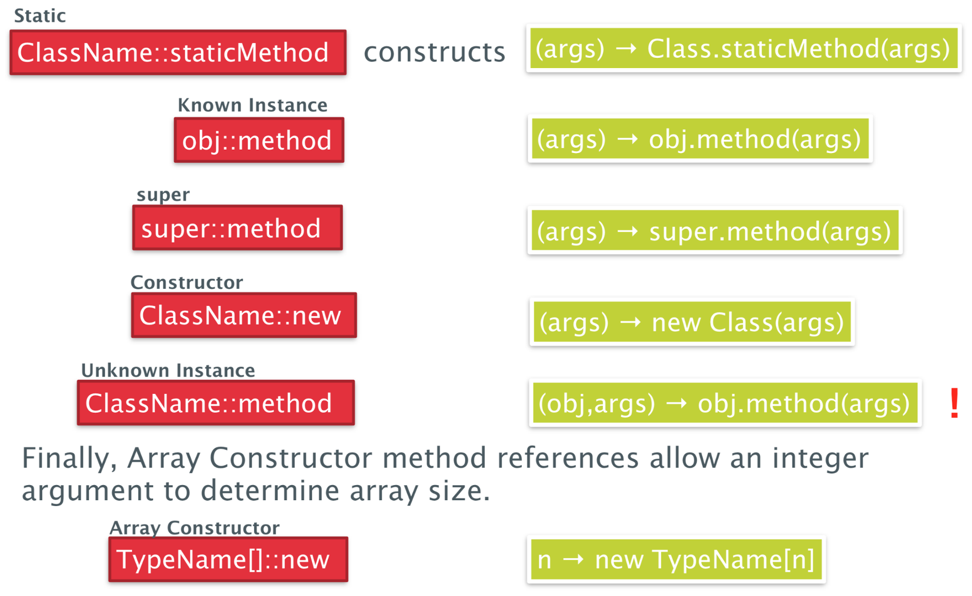
In all cases except of Unknown Instance, it constructs a lambda expression with one argument
For unknown instance, the resulting lambda expression also expects the object reference as an argument

Let’s look at an example for unknown instance
We will define a higher-order function that takes a function and a list of people, then applies that function to each person and prints the output of the function to the console:

private static <T> void listAll(Function<Person, T> f, List<Person> ps) {
for (Person p : ps) {
System.out.println(f.apply(p));
}
}

This is how we could call this function using an unknown instance method reference:

List<Person> people = List.of( ... ); // a list of some people
listAll(Person::getName, people);
listAll(Person::getHeight, people);

Recursion

Finally we will take a brief look at recursion
Anticlimax warning: they aren’t very good
Unfortunately we cannot reference a variable in its own initialiser, like in this example:

class FactNonExample {
static Function<Integer,Integer> f = i -> (i==0)? 1 : i *

f.apply(i-1);
int fact(int n) {
return f.apply(n);
}
}

In order to make this work, we need to wrap the function inside another function which we will call Recursive:

public class FactExample {

private class Recursive<I> {
I f;
}

private Recursive<Function<Integer,Integer>> rec =

new Recursive<>();

public FactExample() {
rec.f = i -> (i==0)? 1 : i * rec.f.apply(i-1);
}

int fact(int n) {
return rec.f.apply(n);
}

}

Programming with Streams

Functional programming and lists

We have list and arrays in Java but these are not like the lists in Haskell
In Haskell, lists are structural and immutable
Furthermore, the way we are used to traverse lists is not quite functional in style
It’s a process that is far too imperative - the traversals are done manually by the client by explicitly navigating the list

External vs internal iteration

When we talk about iteration, there are two different approaches: external and internal iteration

Let’s first look at an example of external iteration:

Iterator it = shapes.getIterator()
while (it.hasNext()){
Shape s = it.next();
s.setColor(Color.RED)
}

This is an example of external iteration because you as a programmer control how the iteration happens
It is your responsibility that you select the next element, check whether there are any more elements left and so on
The enhanced for loop is just syntactic sugar for this

Now look at an example of internal iteration:

shapes.forEach(s -> s.setColor(Color.RED));

This time we do not control how the interaction happens
Instead we just pass a function which is executed on every element of the collection
In other words, you as a programmer just declaratively define what should happen with every element of the collection
The iteration itself happens in the background

Streams in Java

As it turns out we have something in Java which is quite similar to the immutable lists in Haskell
These structures are called streams
They support a number of useful stream operations which can be concatenated in a functional style

There are two types of stream operations
Intermediate stream operations

They are implemented as lazy operations, meaning that the stream values are calculated as they are required
They return another stream
They can be composed with other operations

Terminal stream operations

They are implemented as eager operations, meaning that all of the stream values are calculated
They consume the input stream and produce a side-effect or a return value

Ok this sounds good, but I still don’t really get what a stream is.
No problem, let’s look at a graphical example:

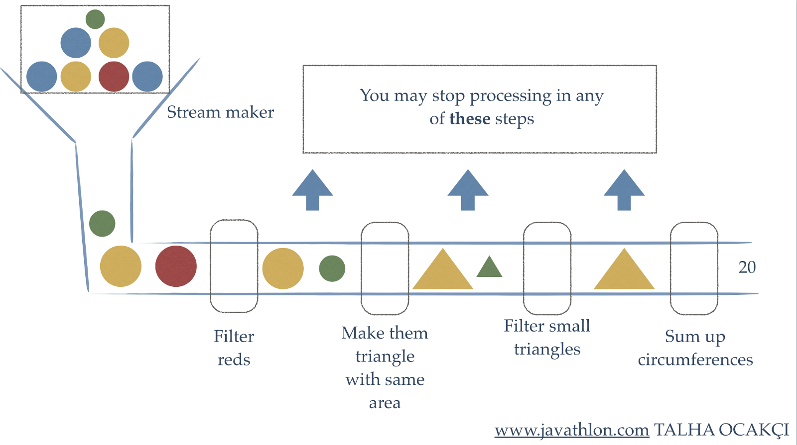
The stream in this graphic is the pipeline
As an input we get a big box of circles. They have different colours and sizes
We need to pour them into the pipe, and by doing that we produce a serial stream of circles
The first intermediate stream operation is “filter reds”

It will take the input stream
It will analyse every circle and throw away all red circles
It will produce an output stream that contains all the remaining balls

The next intermediate stream operation is “make them triangle with same area”

It will inspect the area of each circle and produce a triangle with the same area and colour

The next intermediate stream operation is “filter small triangles”

It will filter out all triangles that are smaller than some defined area

Now we have a terminal stream operation “sum up circumferences”

It will take the input stream
For every element (triangle) it receives, it will calculate the circumference
It will sum up the circumferences and keep doing this until no further element (triangle) is received
It will not produce an output stream, it will produce a number

Now that we have seen a graphic example, let’s switch back to Java
How can we produce a stream from an array or from a collection?

String[] array = ...
Set<String> hash = ...
Stream<String> arrstr = Arrays.stream(array);
Stream<String> hashstr = hash.stream();

So Stream is a generic class, where you denote the type of the contents with the generic parameter
We can also produce a Stream like this:

Stream<Integer> stream = Stream.of(1, 2, 3, 4);

Next we will look at stream operations in Java

Common operations

Map - Streams as Functors

First we will look at the stream operation map, which has the following signature

interface Stream<T> {

<R> Stream<R> map(Function<T, R> mapper);

…

}

It takes a function and applies the function to every element in the stream to produce a new transformed stream
The function takes an unstructured value and produces another unstructured value
It’s a lazy, intermediary operation
Here is an example

Stream.of(1, 2, 3, 4)
.map(num -> num * num)
.forEach(System.out::println); // 1 4 9 16

So what’s going on here?
We are producing a stream containing the numbers 1, 2, 3 and 4
Then we are applying a function to each of the elements, where we multiply the element with itself. This will produce a new stream with modified elements.
Then we are iterating over each of the elements and printing them to the console using a method reference.

This operation essentially makes the Stream a functor!
Why? Because a functor takes a structured value and an unstructured function and produces a new structured value

flatMap - Streams as Monads

Now we will look at the operation flatMap, which has the following signature

interface Stream<T> {
<R> Stream<R> flatMap(Function<T, Stream<R>> mapper);
}

It takes a function and applies the function to every element to produce the new transformed stream.
However, this time the function does not produce an unstructured value but produces a new stream with just that value, i.e. produces a structured value
However, as you can see flatMap returns a Stream and not a Stream with Streams inside.
Therefore, flatMap flattens all the streams the function produces and returns one single flat Stream.

Does this remind you of something?
Well this is exactly what the bind operation of a monad does, so Stream is also a monad!
In fact, Stream.of(...) is equivalent to “pure” in Haskell because it converts an unstructured value into a structured value (into a Stream)

Here is the same example as above, but this time with flatMap:

Stream.of(1, 2, 3, 4)
.flatMap(num -> Stream.of(num * num))
.forEach(System.out::println); // 1 4 9 16

More stream operations yay

We have seen map and flatMap, but there a whole load more stream operations, for example:

Intermediate Operations	filter	Takes a predicate and returns a stream with elements that satisfy the predicate. Haskell Equivalent : filter
	peek	Takes a consumer and returns a stream with the same elements but also feeds each element to the consumer.
	distinct	Returns a stream with duplicate elements removed (it uses .equals for checking equivalency). Haskell Equivalent : nub
	sorted	Returns the stream sorted to their natural order (only for Streams of Comparable elements possible). Haskell Equivalent : sort
	iterate	Takes a unary operator and a start element and produces an infinite stream by repeatedly applying the function. Haskell Equivalent : iterate
Terminal Operations	forEach	Takes a consumer and feeds each element in the stream to it. Unlike peek it does not produce an output stream.
	toArray	Simply converts the stream to an array and closes the stream.
	reduce	Similar to a fold in Haskell. Takes a base element, and a binary operator and applies it element wise across the stream by accumulating the result. Note that no guarantee of order is given.
	max, min, count	Examples of specific reduce operations Haskell Equivalent : maximum, minimum, length
	collect	Converts the stream to a collection according to a specified Collector and closes the stream.

Let’s look at a typical example of using Streams:

List<String> jobs = ps.stream() // Stream<Person>
.map(x -> x.getJobs()) // Stream<Set<String>>
.flatMap(x -> x.stream()) // Stream<String>
.distinct() // Stream<String>
.collect(Collectors.toList()); // List<String>

Suppose that we have an array of people and wish to list all the different jobs people have, but without repeating any jobs
Suppose also that we have a method getJobs() in Person which returns a Set of jobs of this person
Then we can get that list of jobs exactly like shown above.

State of Streams

I have some bad news: We can only use every Stream once
Once we have operated on a Stream object it remembers that and will not allow any further operations
Thus Streams do have state: Either they are fresh or they already have been operated on.
If you try to operate on a Stream twice, like in the following example, then a IllegalStateException will be thrown

Stream<Integer> str = Stream.of(10, 2, 33, 45);
Stream<Integer> strF = str.filter(x -> x < 30 );
Stream<Integer> strM = str.map(x -> x + 5 ); // Exception thrown here

Optional

A method of note in Stream is findFirst
It returns the first element of the stream but interestingly the return type is Optional<T>
An Optional<T> is a wrapper for an object of type T. It can either hold an actual value of T or it can hold nothing (i.e. be empty)

You can check via the method isPresent() if the Optional holds something
In addition, other interesting methods are

Optional<R> map(Function<T, R> f)
Optional<R> flatMap(Function<T, Optional<R> f)

Similarly, these make Optional into a Monad

Optional is the “Maybe” we know from Haskell in Java.

Parallel streams

The streams we have seen so far were all serial streams
However, there also exist parallel streams, which allow parallel processing
You can create such a stream by calling Collection.parallelStream()
However, be careful that the order of elements does not matter when you apply your stream operations
For streams where parallel processing is possible this can greatly improve efficiency

As an example, let’s write a function that determines whether a number is perfect
A perfect number is equal to its sum of factors (not including itself)

public class Perfect {
static boolean perfect(int n){
int factorSum = IntStream.range(1, n)
.filter(x -> (n % x) == 0)
.sum();
return factorSum == n;
}
}

public static void main(String[] args) {
IntStream.range(1,50000)
.parallel()
.filter(Perfect::perfect)
.forEach(i -> System.out.println(i + " is a perfect number." ));
}

The output is the following:

8128 is a perfect number.
6 is a perfect number.
28 is a perfect number.
496 is a perfect number.

Because of the parallel stream, no order is guaranteed

Functional Programming in JavaScript

We’ll briefly look into functional programming in JS
First, let’s compare OOP to FP

Object-Oriented	Functional
Data and the operations upon it are tightly coupled	Data is only loosely coupled to functions
Objects hide their implementation of operations from other objects via their interfaces	Functions hide their implementation, and the language’s abstractions speak to functions and the way they are combined or expressed
The central model for abstraction is the data itself	The central model for abstraction is the function, not the data structure
The central activity is composing new objects and extending existing objects by adding new methods to them	The central activity is writing new functions

In functional programming we describe what we want to achieve, not how we achieve it

Functional vs Imperative Style

For example, we want to write a function that computes the sum of squares of all elements in an array
This is the imperative style, which we can find in methods in OOP:

var sumOfSquares = function(list) {
var result = 0;
for (var i = 0; i < list.length; i++) {
result += square(list[i]);
}
return result;
};
console.log(sumOfSquares([2, 3, 5])); // prints 38

As you can see, the focus of this code is how to actually compute the result

We have to iterate through the list and sum the squares of each element

It focuses on how we produce the square sum of the list

Now look at an example in functional style:

var sumOfSquares = pipe(map(square), reduce(add, 0));
console.log(sumOfSquares([2, 3, 5])); // prints 38

As you can see the focus of this code is what we want to achieve, not how we do it
First it applies a function square to each element of the list

This is what map(square) does

Then it feeds the output of map into the reduce function

This is what pipe(..., …) does

Then it adds all the elements of the list and produces a sum

This is what reduce (add, 0) does
It essentially works like a fold in Haskell

Note that all these functions are supplied by some third-party library, they are not core JS languages features
We will take a look at a third-party library (Rambda) a bit later

Functional Features

What kind of functional features are available in JS?
First-class functions

We can pass around functions
Meaning that we can take a function as an argument or return a function

Lambdas/anonymous functions with closures

We can write lambda expressions
We have full support of closures

Stateless processing
Side-effect free function calls

What’s not available in JS?
Tail recursion
Pattern matching
Lazy evaluation

Functional Programming in JS with Rambda

From now on, we will look into an example of functional programming using the Rambda library
Our example will be a Task List application, which regularly fetches task data from the server.
The data looks like this:

var data = {
result: "SUCCESS",
interfaceVersion: "1.0.3",
requested: "10/17/2013 15:31:20".
lastUpdated: "10/16/2013 10:52:39",
tasks: [
{id: 104, complete: false, priority: "high",
dueDate: "11/29/2013", member: "Scott",
title: "Do something", created: "9/22/2013"},
{id: 105, complete: false, priority: "medium",
dueDate: "11/22/2013", member: "Lena",
title: "Do something else", created: "9/22/2013"},
{id: 107, complete: true, priority: "high",
dueDate: "11/22/2013", member: "Mike",
title: "Fix the foo", created: "9/22/2013"},
{id: 108, complete: false, priority: "low",
dueDate: "11/15/2013", member: "Punam",
title: "Adjust the bar", created: "9/25/2013"},
{id: 110, complete: false, priority: "medium",
dueDate: "11/15/2013", member: "Scott",
title: "Rename everything", created: "10/2/2013"},
{id: 112, complete: true, priority: "high",
dueDate: "11/27/2013", member: "Lena",
title: "Alter all quuxes", created: "10/5/2013"}
// , ...
]
}

So as we can see, we receive a data object with a couple of properties. The most important one is the task property. It contains all tasks of members with some status information

We want to write a function that accepts a member parameter and

fetches the complete data from the server
then it chooses the tasks for that member that are not complete
then it filters out their ids, priorities, titles and due dates
then it sorts the data by due date

The fetch from the server will happen asynchronously, i.e. our application should not block when it waits for the data
Instead we will use promises that will eventually provide the data as soon it is available
We will attach a consumer to a promise via the “.then(...)” function. The consumer function is called with the data as soon as the promise is fulfilled
We can attach multiple consumers which are called one after the other

Iterative Approach

Let’s look at the imperative approach:

We can also write this in an object-oriented approach
However, this will just shift the imperative code into methods of some class
Therefore, the difference between the imperative code and object-oriented code is mostly just organisation

Back to our imperative code: It’s a bit of a lol
It’s very ugly and not very easy to understand/read
Be honest, when you first saw this, you probably thought WTF is going on?!
It would be so much nicer to write it in functional style

We just say what we want
We don’t say how this is done

We could reduce the code a lot and make it much simpler, thus easier to understand
We will shift away the focus from “how it is done” to “what we want to be done”
Let’s convert this code step by step

Get a property

Get all tasks from data
Imperative	Functional
.then(function(data) { return data.tasks; })	.then(get('tasks'))

So what does get(...) do?
It returns a function that takes in an object and returns the specified property of the object
It is defined like this:

var get = curry(function(prop, obj) {
return obj[prop];
});

Curry enables us to partially apply a function, i.e. only substitute some arguments of the function and return a new function containing the remaining arguments.
When we remove the curry function, it would look like this:

var get = function(prop) {
return function(obj) {
return obj[prop];
};
};

Filtering

Filtering tasks by member name - first version

Imperative

Functional

.then(function(tasks) {
var results = [];
for (var i=0, len=tasks.length; i<len; i++)

{
if (tasks[i].member == memberName) {
results.push(tasks[i]);
}
}
return results;
})

.then(filter(function(task) {
return

task.member == memberName;
}))

What does filter(...) do?
It takes a predicate and a list and checks for each element whether the predicate is true or false
It will produce a new list with all elements where the predicate was true
But where is the list argument in the implementation?
Well, it is a curried function, meaning that filter will return a function that takes in a list
Remember that the “then” block will pass the list of tasks to us

Look at how we manually defined the function that checks for the predicate
We can further improve this by writing a function which returns exactly such a function
Let’s call it “propEq” since we want to check whether a property is equal to something
It will take a property and a value and return a function that checks equality like this:

var propEq = function(prop, val) {
return function(obj) {
return obj[prop] === val;
};
}

This is still quite imperative
What we want to do is get some property and then check equality to some value
For “getting some property” we have the function “get”, as we have seen earlier
For checking equality we can use the function “eq”
If we pipe them together, we will get this slick definition:

var propEq = function(prop, val) {
return pipe(get(prop), eq(val));
}

Looks pretty good so far, however it can still be improved
Note how we just take the arguments into “get” and “prop”
We can use a function called use-over to make this even shorter:

var propEq = use(pipe).over(get, eq);

Now we have arrived at our final definition of propEq
Let’s use it in our code:

Filtering tasks by member name - improved version

Imperative

Functional

.then(function(tasks) {
var results = [];
for (var i=0; i<tasks.length; i++)

{
if (tasks[i].member == memberName) {
results.push(tasks[i]);
}
}
return results;
})

.then(filter(

propEq('member', memberName)

))

Rejecting

Rejecting all tasks that are completed
Imperative	Functional
.then(function(tasks) { var results = []; for (var i=0; i<tasks.length; i++) { if (!tasks[i].complete) { results.push(tasks[i]); } } return results; })	.then(reject( propEq('complete', true) ))

This is very similar to “filter”, except that it keeps only those elements where the predicate is false
It is again a curried function that will return another function that takes in the list

New objects from old

Only keep some properties of every task

Imperative

Functional

.then(function(tasks) {
var results = [], task;
for (var i=0; i<tasks.length; i++) {
task = tasks[i];
results.push({
id: task.id,
dueDate: task.dueDate,
title: task.title,
priority: task.priority
})
}
return results;
})

.then(map(pick(

['id', 'dueDate', 'title', 'priority']

)))

We have seen “get” before to get a single property of an object.
Now “pick” is very similar to “get”, but it takes multiple properties out of an existing object and creates a new object
The “map” function will call some function, which is passed as an argument, on every element of a list

Sorting

Sorting tasks by due date
Imperative	Functional
.then(function(tasks) { tasks.sort(function(first, second) { return first.dueDate - second.dueDate; }); return tasks; });	.then(sortBy(get('dueDate')));

sortBy(...) will sort the list according to the key passed in
Again, we need get(...) to extract the due date from every element of the list

Functional Approach

Let’s summarise the functional approach we have seen so far

var propEq = use(pipe).over(get, eq); // TODO: move to library?

var getIncompleteTaskSummariesForMemberFunctional = function(memberName) {
return fetchData()
.then(get('tasks')) // Get a Property
.then(filter(propEq('member', memberName))) // Filtering
.then(reject(propEq('complete', true))) // Rejecting
.then(map(pick(['id', 'dueDate', 'title', 'priority']))) //New Obj
.then(sortBy(get('dueDate'))); // Sorting
};

Now compare this version with the imperative version we had before
This code is much more elegant and simpler than the imperative one

Alright that’s it, you have reached the end of the content
Next section will be a TL;DR ;)

TL;DR

Welcome to the TL;DR section!
Below is a summary of all the above notes. Use these for when you can’t be asked to read the main notes for the millionth time!
However, remember that this is more like a reference guide; it’s designed to jog your memory.
Please try to read the main notes at least once!

Introduction to functional programming

Features of Haskell:

Concise Programs - few keywords, support for scoping by indentation
Powerful Type System - types are inferred by the compiler where possible
List Comprehensions - construct lists by selecting and filtering
Recursive Functions - efficiently implemented, tail recursive
Higher-Order Functions - powerful abstraction mechanism to reuse code
Effectful Functions - allows for side effects such as I/O
Generic Functions - polymorphism for reuse of code
Lazy Evaluation - avoids unnecessary computation, infinite data structures
Equational Reasoning - pure functions have strong correctness properties

Evaluate expressions like this:

5 + 6
or
(+) 5 6

Make a function like this:

[function name] [parameters] = [function body]

Execute a function like this:

[function name] [function parameters]

Standard list functions:

head returns first element from list
tail removes first element from list
length calculates length of a list
!! returns nth element of a list
take returns first n elements of a list
drop removes first n elements of a list
++ appends two lists
sum calculates sum of elements in a list
product calculates product of elements in a list
reverse reverses a list
repeat creates infinite list of repeated elements

Haskell is left associative, so

f a + b is f(a) + b and not f (a + b)

Useful GHCi commands:

:load name loads script name
:reload reload current script
:set editor name sets editor to name
:edit name edit script name
:edit edit current script
:type expr show type of expression
:? show all commands
:quit quit ghci

Name things in lower camelCase, likeThis.

In Haskell, whitespace matters, so your lines need to be at the same column.