50% coursework, 50% exam
Exam: only covers theory part, the book, Long’s part
Coursework: mini project with case study based on real data. You submit a report

Theory

Introduction to ML Technologies (Chapter 1)

Machine Learning is the science (and art) of programming computers so they can learn from data.

There are four models:


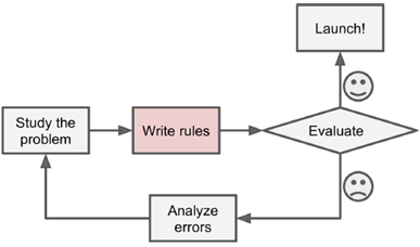
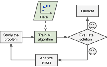
Classical software implementation process: system designer generates rules	Machine learning process: learn from data

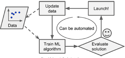
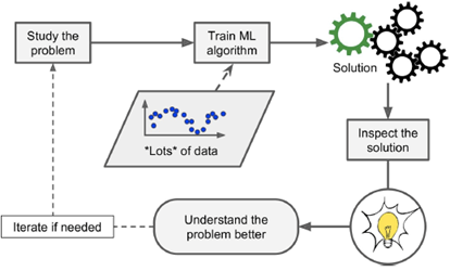
ML with adaptive (changing) environment	ML generates new insights

When there is no solution using the traditional approach...
... you can use machine learning.

ML can also adapt to new data.
You can also get insight about complex problems and large amounts of data (data mining, data science).

Types of ML systems:

Supervised vs unsupervised vs reinforcement
Offline / batch vs online
Instance-based (lazy) vs model-based (eager)

Supervised learning:

Input → Output
Given this → output this
That’s the training data; it’s just a set of correct input-output pairs

Unsupervised learning:

Just input
Try to predict the output
Good for when there’s no absolute “correct” answer

Semi-supervised learning:

A mix between the two

Offline learning:

All inputs are available at the beginning
The machine just crunches the entire data set at one time
The machine outputs in bulk

Online learning:

Data comes into the system through a stream
The machine outputs as a stream
Good for input that depends on earlier output

Instance-based (lazy) learning:

There is no model (it is stateless)
Data points are compared with earlier data points or neighbouring ones
Inputs are computed on the fly
No global parameters are set

Model-based (eager) learning:

A model is set
The machine remembers everything
Data points are compared with the stored model

Parametric model:

Has a predetermined number of parameters set
Degree of freedom is limited, which reduces overfitting (but increases underfitting)
E.g. linear models

Nonparametric model:

Number of parameters is not determined prior to training
More freedom than parametric models, so overfitting is more likely
Should use regularisation to limit the model’s power and reduce overfitting
E.g. decision trees

Data issues:

Not enough data
Non-representative data (e.g. bias)
Poor quality data

Algorithmic issues:

Feature selection (too many features)
Overfitting (too specific; not general enough)
Underfitting (too general, not specific enough)

Overfitting:

High accuracy on training data, low quality on prediction
This happens because of “noise” in the data points (the data isn’t perfect)
Your machine captures the noise of the data and not the underlying input-output relationship

Main problems of machine learning:

Insufficient quantity of training data
Nonrepresentative training data
Poor-quality data
Irrelevant features
Overfitting the training data
Underfitting the training data

When you have two models, pick the simpler one. This is Occam’s razor.

So how do we test ML algorithms?
Half the data; use half for training and the other half for testing.
Why not swap the training and testing halves? We’ll reduce average generalisation errors.
This leads into the K-fold cross validation:

We partition the data into K pieces.
Train with K - 1 partitions, and test with the last one.
Repeat this K times, using a different, unique testing partition for every iteration.
You usually use around 5 or 10 for K.

Classification (Chapter 3)

Classification: take raw data, understand what the raw data is about and put it into one of a finite number of categories
Is it a shape? A chair? A table?
It’s the most fundamental step.
A more serious example is a bank deciding if your card usage was fraudulent or not.

Two kinds of classification:

Top down: Inspiration from higher abstraction levels
Bottom up: Inspiration from biology, e.g. neural networks

Classification algorithms:

Support Vector Machines (SVMs)
Decision trees
Deep neural nets

Binary classifiers:

Only two options (yes/no, 1/0, red/blue, hamon/stands etc.)
Examples:

Spam filters
Fraud detection
Object detection

Performance measures

How good is our algorithm?
Factors (used in regression models):

Root Mean Square Error (RMSE) - If you plot the RMSE you can differentiate it everywhere
Mean Absolute Error (MAE) - You cannot differentiate the MAE at the turning point
Because RMSE squares the errors it penalises larger errors more than MAE, which is useful when large errors are particularly undesirable

The smaller the error the more accurate

Why accuracy as a performance metric sucks

Example: asthma attack prediction from cough sound
99%: no attack
1%: attack
We use a ML algorithm to do prediction and it’s 99% accurate.
Is that good?
We have a dumb algorithm that always says no.
What’s the accuracy of that?
It’s 99% again, because 99% of the time it’ll be correct.
So our stupid algorithm is just as good as our fancy ML algorithm. Not good!

Confusion matrix:

True positive (TP): “yes”, correctly predicted as “yes”
True negative (TN) “no”, correctly predicted as “no”
False positive (FP) “no” incorrectly predicted as “yes” (Type I error)
False negative (FN) “yes” incorrectly predicted as “no” (Type II error)
Example:

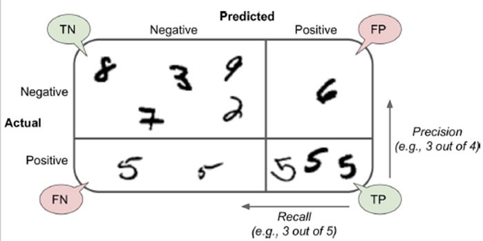
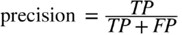
Ratio of correct ones among “yes” predictions

“Did we only predict the ‘yes’ that we should have predicted?”

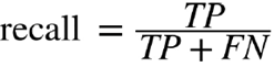
Ratio of “yes” that were successfully predicted

“Did we predict all the ‘yes’ that we should have predicted?”

Now let’s use this on our stupid algorithm:

Precision = 0 / (0 + 0) = NaN
Recall: 0 / (0 + 0.1) = 0

Basically, this algorithm sucks (but now we can prove it with numbers).

“But these are two numbers! I’m lazy and only want one number”
Then we can use F-score (F1). It’s the harmonic mean of the two.

However, F1 is only high if both precision and recall are high.
It’s not good if you have high precision + low recall or vice versa.
It’s also not good if we only want high precision or only want high recall.

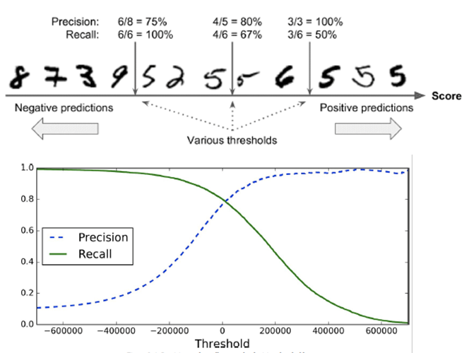
So how do we set the parameters for precision / recall trade-off?
We can use a threshold used in SGDClassifier (stochastic gradient descent) from scikit-learn where lower means we want high recall, and higher means we want high precision.

ROC (receiver operating characteristic) curve:

Like a precision / recall curve, but instead we plot true positive rate (TPR, or recall) against false positive rate (FPR)
What’s FPR? It’s the ratio of negative instances incorrectly classified as positive. It’s 1 - true negative rate (TNR), which is the ratio of negative instances correctly classified as negative.
TNR is also called specificity.
So basically ROC curve is recall against 1 - specificity.

So what do we do with this curve?
Find the area under the curve (AUC).
If the AUC is 1, our classifier is perfect.
A purely random one will have an AUC of 0.5.
Now we have another metric to measure performance.

Multiclass classification:

We have more than two classes
Some classifiers can handle this normally (e.g. random forest, naive Bayes)
Others need modifications, like SVMs
One-versus-all (OvA):

We use one classifier for each class
Each classifier predicts with a confidence score (e.g. 0 - 100%) to which degree the input matches the class
We run each input through all classifiers and each classifier predicts some confidence score
The final outcome for a given input is the class for which the highest confidence score was predicted
Example: Given pictures of fruit, is it an apple, a banana or a kiwi?
We have 3 classifiers, which output a confidence score (0 - 100%) for their class
Classifier 1: Is this an apple (or something else)?
Classifier 2: Is this a banana (or something else)?
Classifier 3: Is this a kiwi (or something else)?
E.g. for one input we get outputs 60%, 55%, 65%, therefore the final decision is kiwi

One-versus-one (OvO):

We use one binary classifier for every pair of categories
“Binary” means that each classifier predicts either one or the other class (e.g. “A” or “B”) instead of outputting a confidence score
For n classes we need a total of classifiers
In most cases (where n > 3) we need more computations, but easier to scale with large training data sets as we train each classifier only on a subset that contains those classes
We run each input through all classifiers and select the class that was predicted most frequently as the final answer
Reusing the fruit example from above, we need the following classifiers:
Classifier 1: Is this an apple or a banana?
Classifier 2: Is this an apple or a kiwi?
Classifier 3: Is this a banana or a kiwi?
E.g. for one input we get outputs “apple”, “apple” and “kiwi”, therefore the final decision is “apple”

Multilabel classification:

We can also assign multiple categories / labels to data.
Not all classifiers can support multilabel classification

Multi-output classification:

Multilabel + multiclass

Regression (Chapter 4)

Classification was discrete label values:

Is it a cat?
Is the person wearing a hat?

What if the output is continuous / unbounded?

Tomorrow’s highest temperature
Students’ final marks

We use regression models!

Linear regression

Linear correlation between two features X and Y (with some noise) can be modelled with a straight line

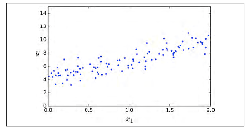
We can have more than two features
In general, linear regression follows this formula:

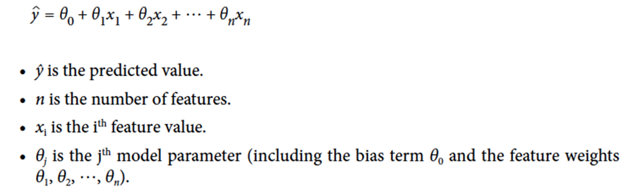
You can also represent this with vectors:

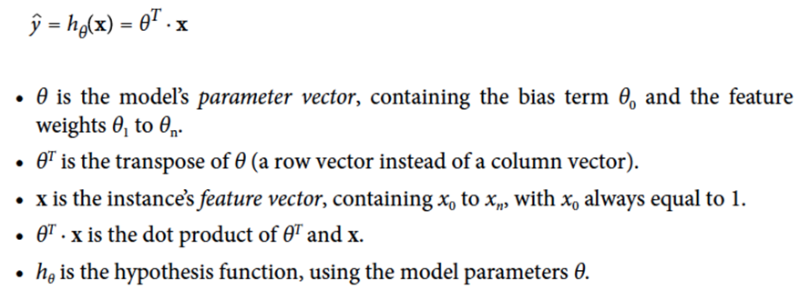
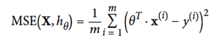
How can we compute the error of our regression model?
We can use MSE (mean squared error):

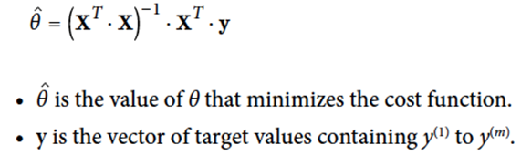
So how do we pick the best theta values that minimises the error function the most?
We use the normal equation!

But in the real world, x is very large, so using this is infeasible.

Polynomial regression

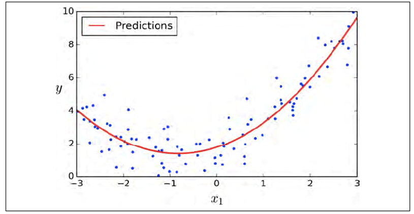
Sometimes, we cannot model a correlation (e.g. between x and y) using a straight line
You can model it with a curve

But polynomials can have any power.
What power do we use? 300? 2? 1?

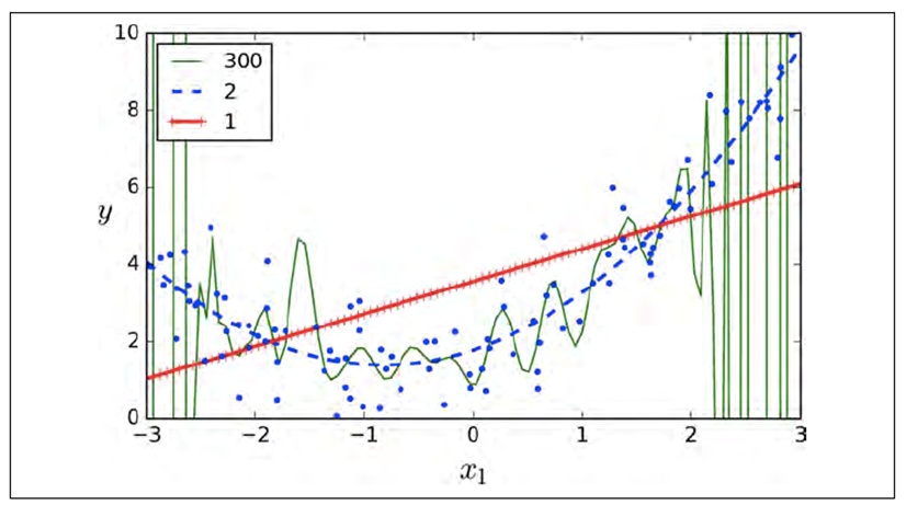
It seems 300 is too big and 1 is too small.
Too big = overfitting
Too small = underfitting

Regularisation

How do we know our model suffers from underfitting?
Well, here’s one:

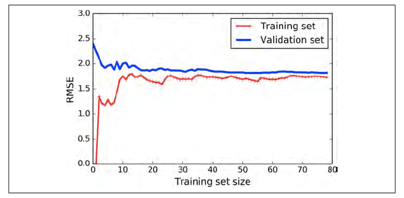
When the size increases, it converges to a large value (in this case, around 1.75).
When that happens, the model is underfitting.
If it’s underfitting, it’s not complex enough.
How do we fix that? We make it more complex!

What about overfitting? How do we know if our model is doing that?
Here’s one:

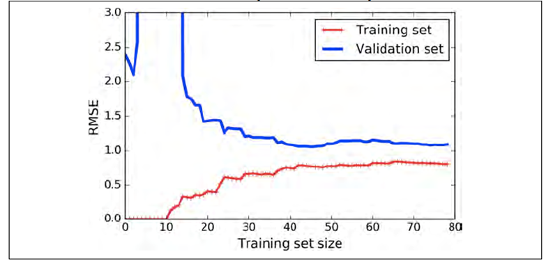
Look how far apart the blue and red lines are when the training set size increases.
There is a big gap in loss between the training and validation data sets!
When that happens, the model is overfitting.
How do we fix that? We make the model less complex!

How do we control overfitting / underfitting?
We use regularisation, which is basically limiting the freedom of the model to avoid overfitting / underfitting.
The principle comes from Occam’s razor (basically, pick the simplest one)
We capture model complexity in the cost function (cost function = loss + model complexity)
In other words, we are adding a penalty to the cost function.
There are different types of “penalties” to use:

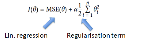
Ridge regression (Tikhonov regularisation): MSE of linear regression + regularisation term

Ridge tries to keep the weights as small as possible.
α (alpha) is a hyperparameter for Ridge. If it’s 0, Ridge is the same as linear regression. If it’s 1, all the weights will be very close to 0 and the result is a flat line through the data’s mean.
If we’re underfitting (we have high bias), reduce alpha.

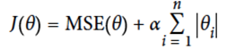
Lasso (Least Absolute Shrinkage and Selection Operator Regression)

We use Lasso when we are sure the correct model is sparse (most of the weights are 0 except the few features that actually matter)

Elastic net

Behaves less erratic than Lasso.
If you want Lasso without erratic behaviour, set l1_ratio close to 1.

Gradient Descent

We can use this to find the theta value that gives the minimum error:

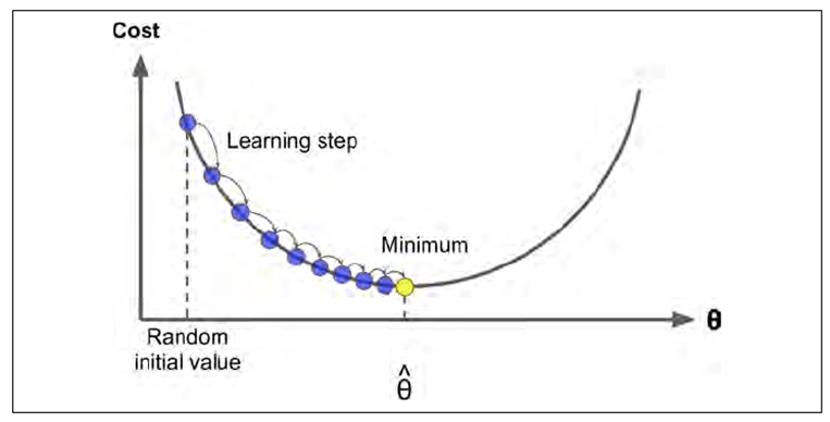
Ok, what’s going on here? There’s some blue dots and a yellow dot and a curve and aaaaah
Basically we’re using (batch) gradient descent to find the minimum theta value for our model

We pick a random point on the curve
We get the gradient on that point
We travel down the gradient using one of these regularisation equations
Find the new point on the curve and repeat until we’re at the bottom

The problem with GD is that it uses every single data point for each step we take, which can get computationally expensive.
However, it scales well with features: if we have loads and loads of features, GD will perform way better than the Normal Equation.

Gradient descent cannot get stuck at a local minimum because the MSE cost function for Linear Regression is convex, i.e. there only exists one global minimum.

A convex function, as opposed to a concave function.

As you can see, if our graph looks like the one on the left, there’ll only be one global minimum.

Again, we don’t live in a perfect world; this would take too long in a real use-case!
What do we do? Do we just give up? Is life really worthless after all?
No! We use stochastic gradient descent (SGD)
What’s that?
Basically, when we compute the gradients we don’t use all the data points, we only use one data point for each feature.
This drastically reduces the amount of computation if we have loads of training data, making it the fastest gradient descent algorithm (it will reach the optimum faster than GD and mini-batch GD)
The result is similar to simulated annealing (remember that?)
Because of how erratic SGD is, the error is going to bounce up and down, but on average it’ll eventually converge to the optimum.
However, it won’t actually reach the optimum; it’ll just bounce around it...
... unless you slowly reduce the learning rate as we approach the optimum (again, like simulated annealing)

There’s also mini-batch gradient descent, which is like SGD but instead of using one data point for each feature, we use a subset of data points.
It’s less erratic than SGD but you get the best of both worlds.

We can also use regression as a classifier using a logistic function

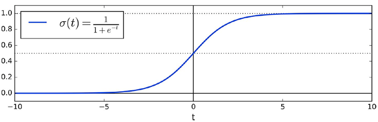
We’re basically converting continuous to discrete categories.

Softmax regression

Softmax is simply a way of doing multiclass classification with a regression algorithm.
It works like this:

For every instance x, compute a softmax score sk(x) for each category k

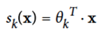
Estimate the probability of x being each class k using the softmax function to the scores

Pick the class with the highest probability for x

You can use softmax for stuff like estimating colours, for example:

if you have a red flower you might get a result like 90% red, 5% blue, 5% green
if you have a turquoise gemstone you might get a result like 56% green, 39% blue, 5% red

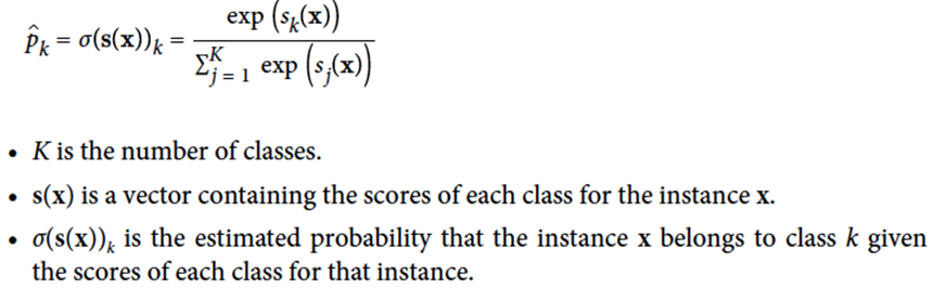
SVMs (Chapter 5)

Let’s say you’re training a ML algorithm that classifies iris plants into the setosa and versicolor species.

We use two features, “petal length” and “petal width”.
When we plot our training dataset as yellow and blue dots we can see that we can separate the two species in different ways, e.g. with the red line or with the purple line below.

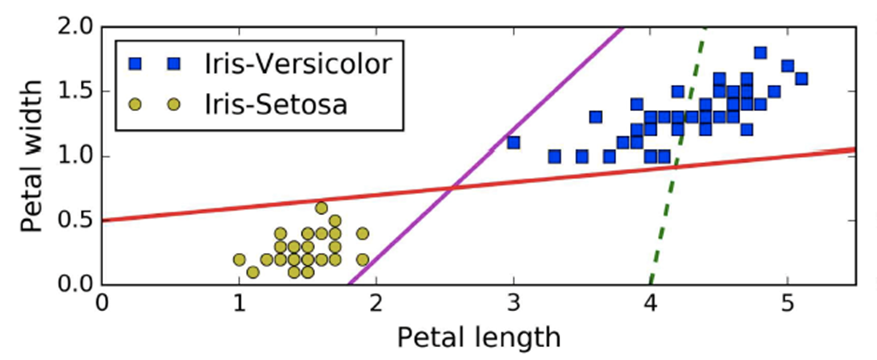
Yeah, those red and purple lines seem to work.
However, they are very close to the data points and thus it’s unlikely that they work well with testing data because only a slightly different position of the data points will result in lots of wrong classifications.
How about using this black line model below instead?

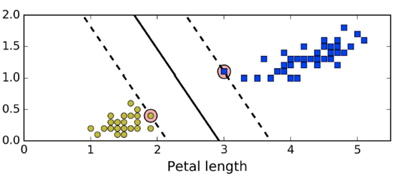
We made our model more general to make it more effective across different inputs, which is called “generalisation”.
That’s the intuition behind SVMs: our model needs to be distanced from the data points.
Take a look at the black line model. It’s not close to any of the data points, and the dotted lines show the boundaries the model should lie in (called the margin).
These dotted lines define the “widest possible street between the classes”, called the wide margin.
By supporting our margin using data lying on the edge, we are using support vectors, which are instances located on the street, including the border.

Support Vector Machines (SVM) are models that use this technique.

So, basically, support vector classifiers / machines are classifications with wide margins and is fully determined by support vectors (data on the edge of the margin).
How wide should the margin be, and what happens with the data within the margin?

Initial step: feature scaling

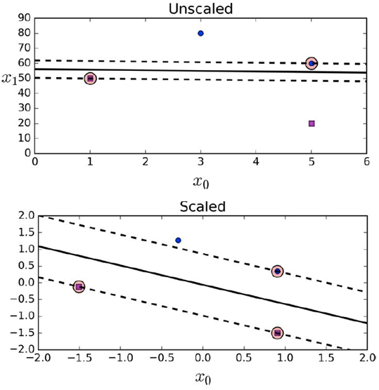
SVMs will try to fit the largest possible separating margin between the classes.
If the data is not scaled, the SVM will neglect small features.

There are two types of margins in SVMs: hard margin and soft margin
Hard margin: no data points can be in the margin (no violations)
Here is a case where a hard margin is impossible (because we will always have violations)

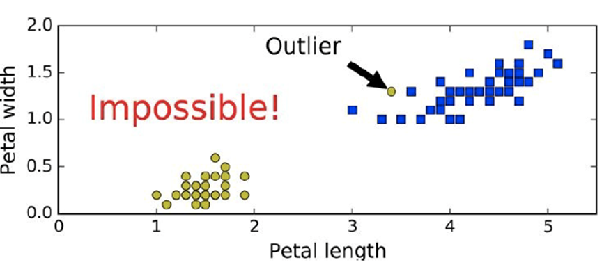
When we have linearly non-separable data like shown above, we cannot have a hard margin!
If we have linearly separable data a hard margin looks like this

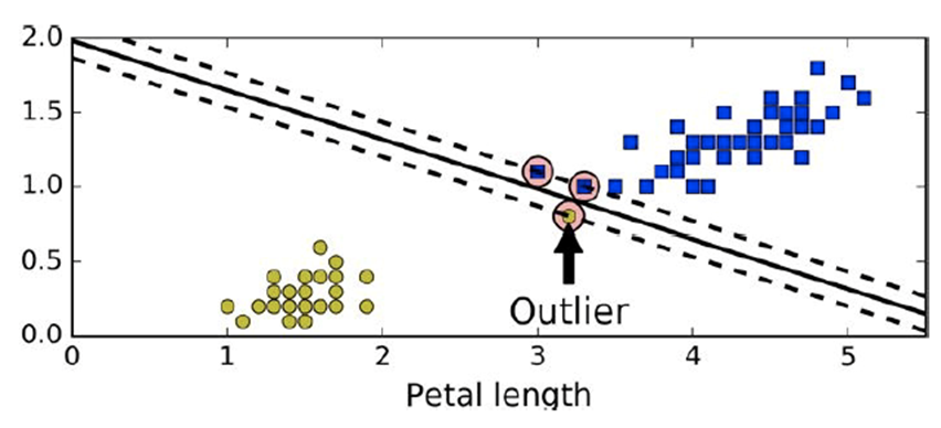
Because of the outlier point, the margin becomes very narrow

Soft margin: data points can be within the margin (we allow violations)
However, we need to try and minimise the number of violations

When using a soft margin, we need a balance of margin width and violations
In scikit-learn, there’s a hyperparameter called C
Small C = wider margin but higher violations
Large C = smaller margin but low violations (low generalisation power)

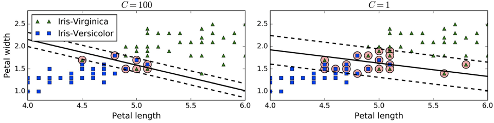
If you’re overfitting, reduce C (make margin wider)
If you’re underfitting, increase C (make margin more narrow)

What if you cannot linearly separate your data, like this:

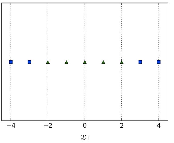
It looks like we need some kind of curve...
We could also add a new “polynomial” feature by mapping our data points to a new dimension, like this

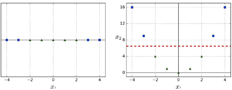
This is called feature space transformation.
In this example, we square each of our data points.
By turning our data into a curve, now we can just use one line to model our algorithm!
If it helps you to visualise it, you could say we’re “moving” the curve from our algorithm to the data itself, so instead of our algorithm being a curve, we make our data a curve.
If that just confuses you more, then pretend I never said it.

This is a non-linear SVM.

In scikit-learn, we have a parameter d which is the degree of expansion.
For example:

If we have features a and b, and our degree of expansion d = 3, then our combinations are:

a^3
b^3
a^2 b
a b^2

In general, the number of added features is:

where n is the number of features we currently have

But squaring the data points is boring. Where’s a more interesting, colourful, cool-looking example?

Whoa!

If you set d too low you’ll be underfitting
If you set d too high you’ll be there all day
What are we going to do?
We use magic!
It’s actually the Kernel method. It makes it possible to get the same result as if you added many polynomial features, even with very high-degree polynomials, without actually having to add them.
Basically, just add kernel=”poly” to the SVC function in scikit-learn.
But for linearly separable data models, just use normal LinearSVC because it’s easier! Use this for non-linear data.

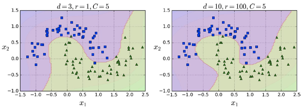
Here’s the trick in practice:

The higher the degree, the more non-linear it is.
The parameter “r” means how much the model is influenced by high-degree polynomials vs low-degree ones (so it’s kind of like a coefficient)
However, d and C are the easier parameters to set.

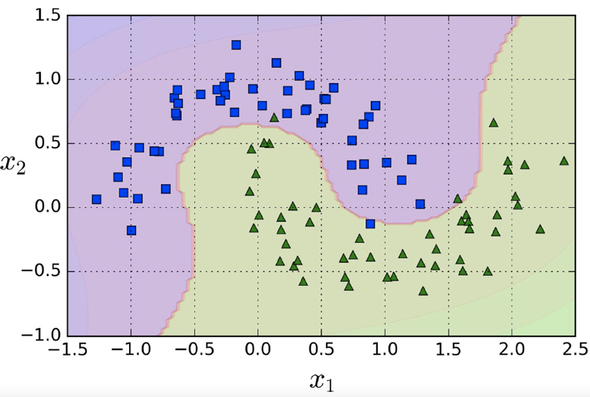
You wanna see more magic?
Ever heard of Radial Basis Functions (RBF)?
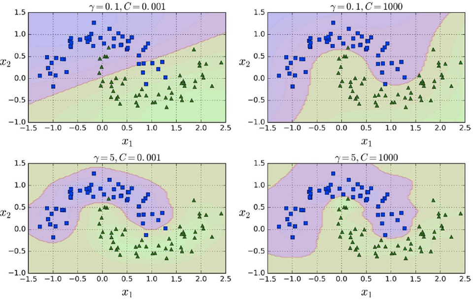
It goes like this:

You set some points as landmarks, position some similarity functions on those landmarks

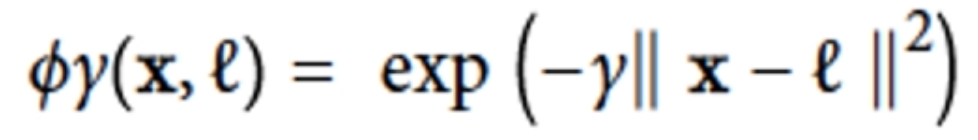
As a similarity function we use the Gaussian radial basis function which evaluates to a value between 0 and 1

The similarity function on the landmark itself is going to evaluate to 1 (because it’s exactly the same point)

You then evaluate the similarity functions on every data point
You use those values as the new feature values (instead of using the original values)

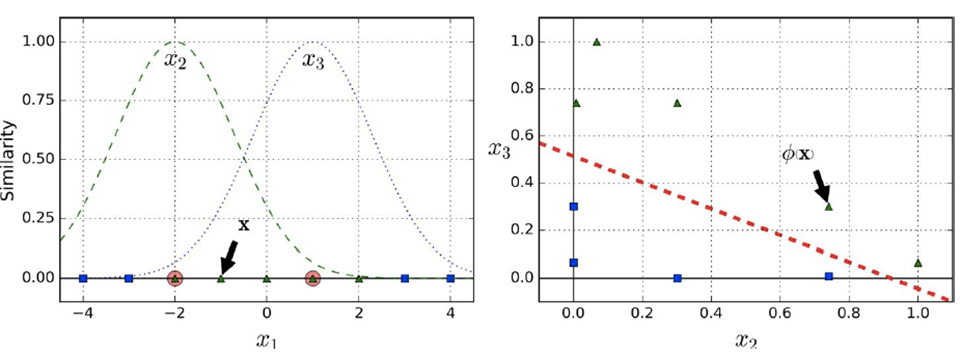
It uses a hyperparameter “gamma”.
Increasing gamma makes the bell-shaped curve narrower, so each instance’s range of influence gets smaller.
Decreasing gamma makes the bell-shaped curve wider, so the range of influence gets bigger and the decision boundary gets smoother.
Like C, you should decrease it if you’re overfitting and increase it if you’re underfitting.

How do you pick the landmarks? I don’t know; pick whatever ones you want. Trial and error.

For example, we have a feature x1 and pick two similarity functions which evaluate to features x2 and x3
After evaluating the similarity functions we can use a line to separate the blue rectangles from the green triangles (see graphs below)

Again, we need a balance of similarity features: too few, and it can’t handle the complexity. Too much and the computational time will be too big.

Ok cool, but where are the pretty pictures?
They’re here:

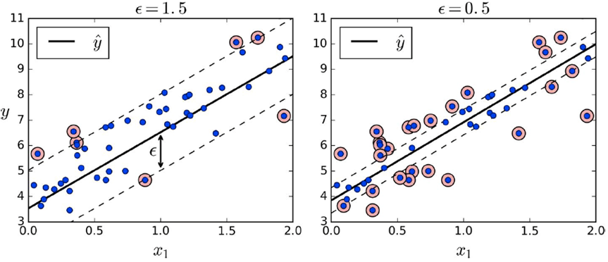
So this is all for classification, but we can use this for regression as well!
Instead of finding a separator, now we want to find the narrowest stripe that contains all the data.
The width of the street is controlled by the hyperparameter epsilon.

Decision trees (Chapter 6)

This topic was also covered in Intelligent Systems up to Gini scores, but it’s still worth reading for the extra ML bits.
The topics already covered in Intelligent Systems will be bare-bones summaries below, so if you need a more in-depth refresher, go on the link!

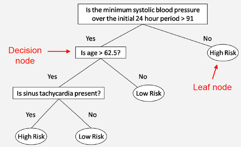
Decision tree: takes a series of inputs defining a situation, then outputs a binary decision / classification
Decision trees check features of inputs in a specific order, or just enough information to decide on an answer.
We use observable features to predict an outcome.

Typically, decision trees are binary trees, like you see above, and they usually become balanced at the end of training.
So if you have n training data instances, the approximate depth would be log2(n).
The problem we have is: what’s the most optimal / efficient order of checking the features?

The idea is to pick the next feature whose value will reduce the most uncertainty about the output.
There’s two ways to do this:

Pick the feature that will give us the most information about our data (highest information gain)
Pick the feature that has the highest Gini score improvement

How do we measure information gain?
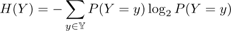
We use entropy and conditional entropy.
Entropy: A measure of the amount of disorder or uncertainty in a system

Tidy room => low entropy, low uncertainty (to find stuff)
Messy room => high entropy, high uncertainty (to find stuff)

So, basically, we want to reduce this value.

If you need a better refresher on entropy, look at the Intelligent Systems notes.

Conditional entropy: the level of uncertainty, given that some event is true

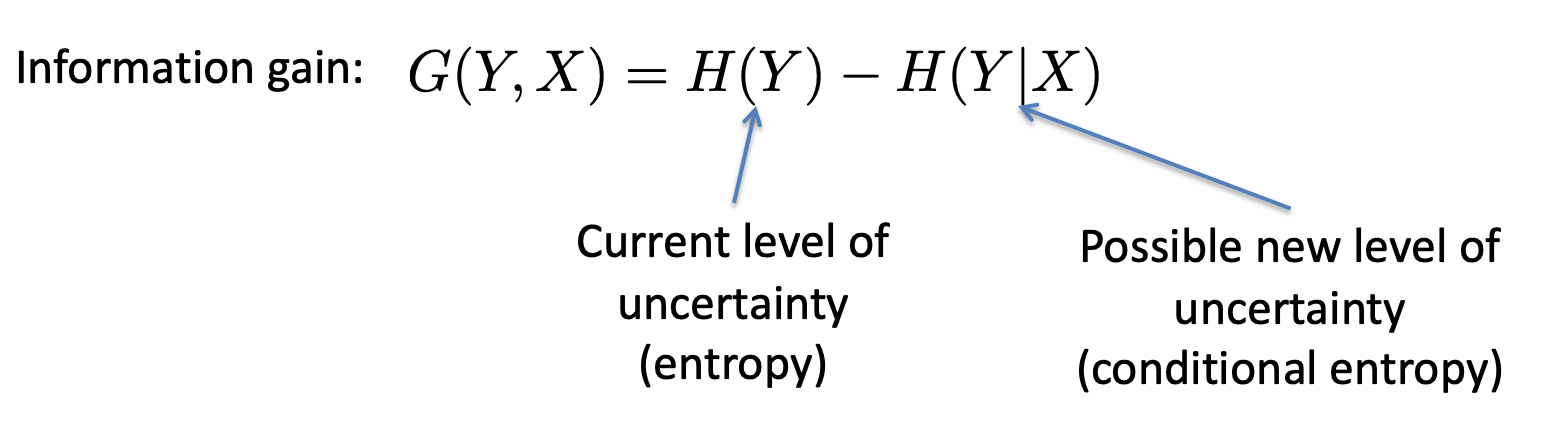
Information gain: how much info we will gain if we query this attribute
In other words, how much uncertainty / entropy we will clear away if we query this attribute

Now that we have this, we just need to pick the attribute with the highest information gain.

Keep in mind that scaling the input will not improve performance of the decision tree model. Decision trees don’t care about the scale of the input, so scaling the input will be a waste of time.

If your decision tree is underfitting:

Increase maximum depth
Decrease minimum samples per leaf
Increase number of features

Time complexity of a decision tree:

n is the number of features
m is the number of training instances

Decision trees also have a presort option, which is only helpful for datasets smaller than a few thousand instances.
Any bigger and the presort option will slow down training instead.

Gini score: the ratio of a certain type of data point amongst others in a class when you half a tree by some feature.

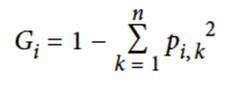
The smaller the Gini score, the more homogenous the class is (the less diverse it is)
That means that class will be more certain about what features its data will have

Typically, a node’s Gini score is lower than its parents.
This is ensured by the training algorithm, as we want the nodes with the highest Gini score to be split first (we want the highest information gain at the start).

Algorithm:

Choose the feature that provides the lowest of the (weighted) sum of the Gini score of the children nodes
Repeat until reaching leaf node (e.g. Gini score is very small)

Scikit-learn uses the gini score instead of information gain
Using the iris flower dataset, we create a decision tree that uses the petal length and width as two features
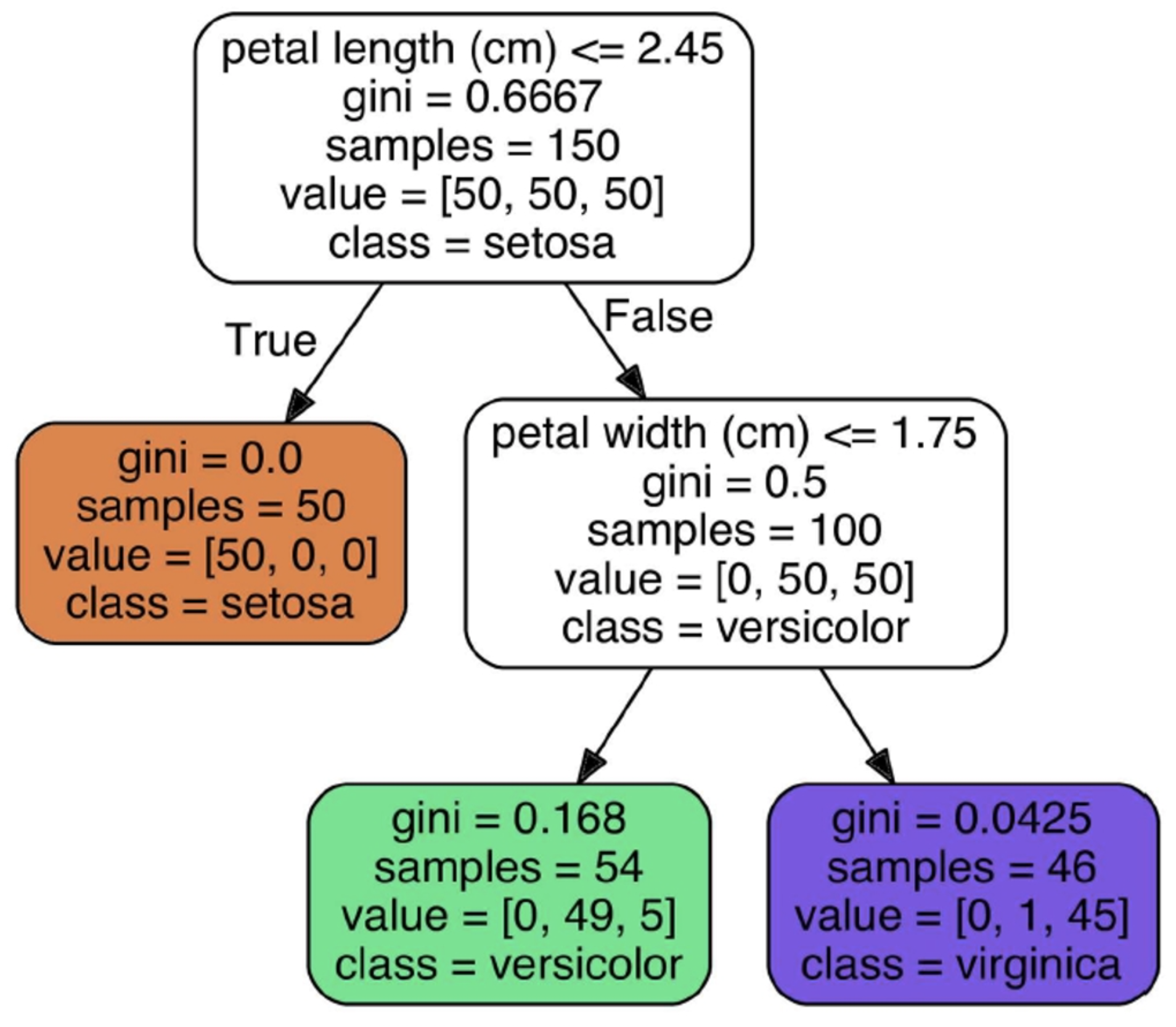
At first, the gini score is high but it approaches 0 as our tree becomes deeper
At some point, when the gini score is low enough, we can stop
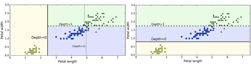
Here is a plot of our decision tree with the data points

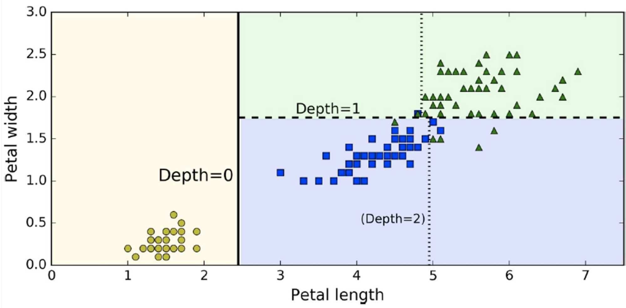
Decision trees don’t know the depth of the tree before training, so they can easily become overfitted.

For example, in this image, it’s a bit too specific for the training data.
This is what it should be:

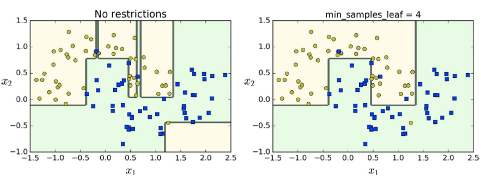
By regularising the decision tree, the model will generalise more (which reduces overfitting)
In this example, we restrict the minimum number of samples per leaf to 4

We can also use decision trees for regression, too (predicting values instead of classes)
We need to set max depth values though

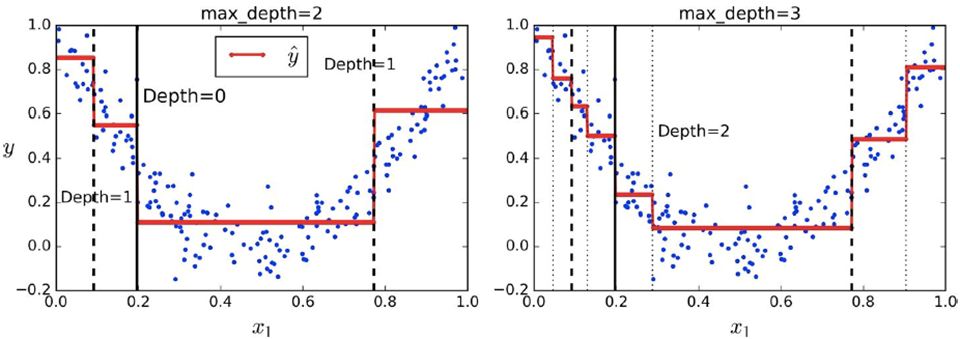
This time, the splitting (red) line will be the output of our model
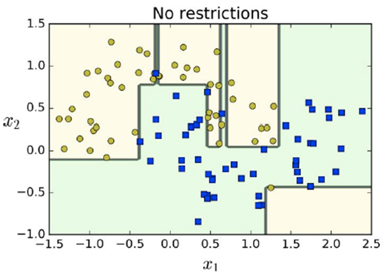
When we don’t have any restrictions overfitting can occur easily
We should introduce restrictions (regularisation) to achieve generalisation

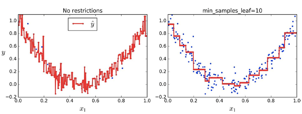
You can see how much overfitting the model does if there is no regularisation

Instability: the model is very sensitive in terms of the data
A big drawback of decision trees
For example, look at the different decision trees before and after removing a single data point from the training set:

It does this for rescaling or rotation as well

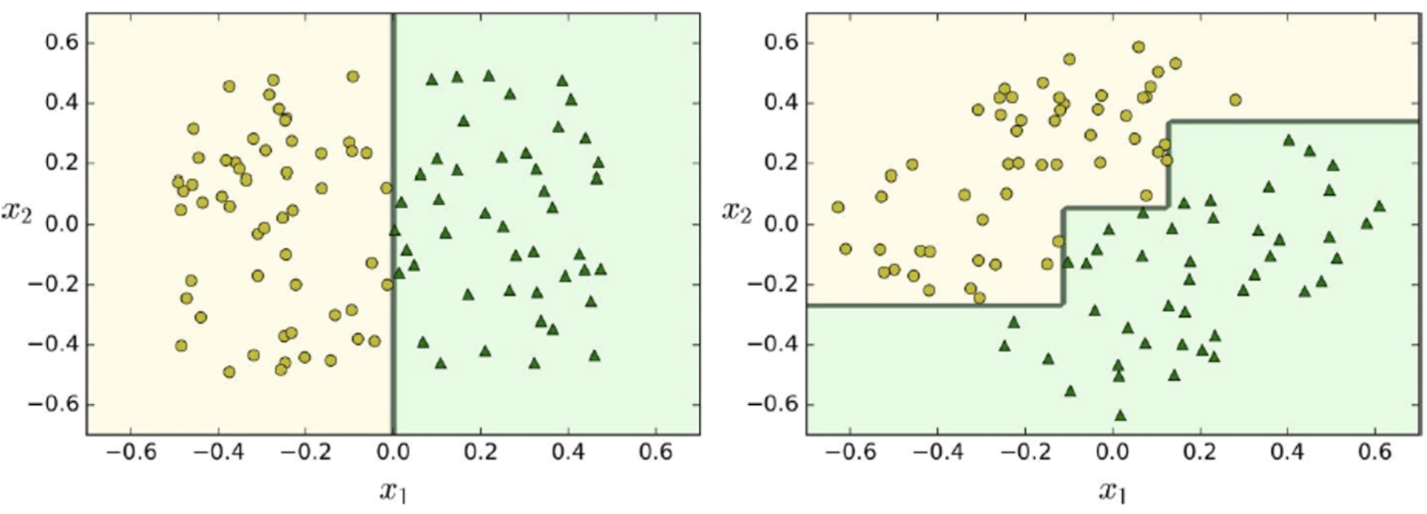
This is the same dataset but rotated.
Decision trees are like this because boundaries are typically orthogonal to the dimensions, meaning the method is not stable and robust.
We can fix this using ensemble learning!

Ensemble learning (Chapter 7)

A single classifier can train on one single data model and yield one result.

A lonely classifier, all on its own.

What if we had a whole load of classifiers?

Whoa! It has loads of friends now!

If one classifier can only yield a 51% accuracy, then why not use a bunch of classifiers and aggregate their results using a majority vote or something?
It’ll work better because of the law of large numbers!

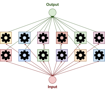
All of its friends work together by forming their own results and then aggregating them.

Voting

There are two types of voting: HARD VOTING and soft voting.

Hard voting is simply a majority vote.
If two classifiers voted “real” and one voted “fake”, the overall choice will be “real”.

Soft voting is used when classifiers can output class probabilities.
For example, a classifier could say it’s 70% likely to be real and 30% likely to be fake.
Soft voting will pick the class with the highest probability average.
For example:

Classifier 1: 70% real, 30% fake
Classifier 2: 40% real, 60% fake
Average real = (70 + 40) / 2 = 55
Average fake = (30 + 60) / 2 = 45
Overall class = real

Before I move on to bagging and pasting, here are some common practices:

Classifiers should be independent (correlated classifiers don’t work well together, because they’ll make the same mistakes)
Ensemble completely different classifiers
Vary the training data (using bagging and pasting)
Vary the feature sets (random patches & random subspaces)

Bagging and pasting

How do we split up the data to all the classifiers? Do we just give every classifier all the data?
No! If we did that, all the classifiers would yield the same results.
Instead, we randomly sample the data to train each classifier.
There’s two ways to do this, called bagging and pasting.

Bagging (bootstrap aggregating): choose with replacement

We can sample the same data point for multiple classifiers
If our data set is D1, D2, D3, D4, then our classifiers could get:
C1: D1, D2
C2: D2, D3
C3: D3, D4

Pasting: choose without replacement

When one classifier gets a data point, it’s reserved just for that classifier.
If our dataset is D1, D2, D3, D4, then our classifiers could get:
C1: D1, D2
C2: D3, D4

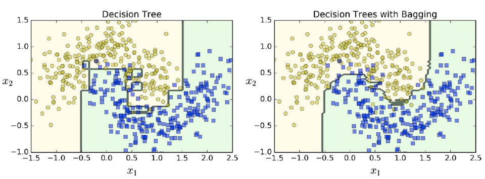
Here’s the difference between using a single decision tree vs. using multiple decision trees with bagging:

Random

Why sample just the data; why not sample the features too?
Random patches method: sample both the training data and the features
Random subspaces method: just sample the features and keep all data

When you ensemble multiple decision trees, you get a random forest.
Get it? Because you’ve got lots of trees, it makes a forest?
It typically uses bagging.
It’s a random forest because only a random subset of features is considered for each split, so random forests are RNG-based.
The most important features appear closer to the root, so you can tell which features are the most important by the average depth at which that feature will appear.

Extremely Randomised Trees takes things even further!
Normal decision trees in random forests use a “best, most discriminative threshold” when deciding on a feature to split with.
Extremely randomised trees use a random threshold for each candidate feature, and the feature with the best random threshold is picked.
This reduces variance for greater bias.

Boosting

What? There’s some kind of stat boost we can apply to our model to make it perform better?
Uh, not really. Boosting (hypothesis boosting) is the sequential combination of classifiers.
So instead of lots of classifiers working in parallel, the classifiers work one after the other in a giant chain.

Ensemble learning	Boosting

There’s two main boosting techniques:
AdaBoost

Assign a weight to each data point in the training set

The weights tell the classifiers how important this data point is.
Initially, this weight will be the same value for each data point.
All weights add up to 1

Train the first classifier on some features of the whole data set

Often, a decision tree is used as a classifier
Often, only a single feature is chosen (so the depth of the tree is 1)
Because a single classifier has very limited power on its own we call it a weak classifier (because it's crap on its own)

Identify the wrongly classified data points and adjust the weights

If a data point was classified correctly we will reduce its weight
If a data point was classified incorrectly we will increase its weight (“boosting” its weight)

Train the following (second) classifier on other features, taking into account the weights

By taking the weight into account we try to correct the mistakes (wrongly classified data points) from the previous classifier
We try to get correct predictions on data points that have higher weight compared to those with lower weight

Repeat step 3 and 4 until you exhausted the feature space, used a desired number of predictors or you are happy with the final output

Basically, we use loads of weak classifiers to make a really good overall classifier

If your AdaBoost ensemble underfits, try:

increasing the number of estimators
reducing the regularization hyperparameters of the base estimators
slightly increasing the learning rate.

Gradient Boosting

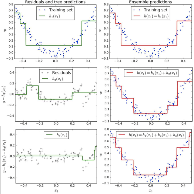
Train a model (e.g. a regressor) on the training set
Use the model to predict the training set and calculate the error

The error is the difference between the expected value (given as part of the training set) and the predicted value

Train the next model on the error of the previous model
Calculate the new error between the prediction and the old error
Repeat steps 3 and 4 until you used a desired number of predictors or you are happy with the final result

Here’s some graphs that show boosting:

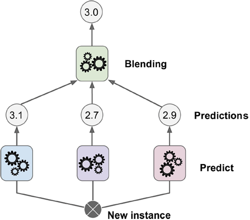
Stacking

Instead of using an aggregation function like majority vote, why not use another ML model to learn how to aggregate?
This is called stacking.

Dimensionality reduction (Chapter 8)

Curse of dimensionality

An extreme point is a point at most 0.001 units away from a border
In a unit square, a point has 0.4% chance of being an extreme point.
In a 10,000-dimension hypercube, there is a 99.999999% chance of being an extreme point.
The key point here is that it becomes much easier to be an extreme point with a higher number of dimensions, meaning that overfitting is way easier.

In addition, having higher dimensions make the data more sparse, meaning data is really spread out.
That means more data is needed to reach a good density and properly train our models and we have more noise which will lead to overfitting.
Example: 100 dim data (i.e., data with 100 features) needs more data than the number of atoms in the universe to reach an average distance of 0.1
Basically, big dimension bad.

That’s not good!
What do we do? Cry and send some applications to Sainsburys?
No! Don’t worry, this is called the curse of dimensionality: the fact that many problems that do not exist in low-dimensional space arise in high-dimensional space.

So how do we lift this curse? Is there a level 20 priest who can use Remove Curse?
No need! There’s methods to reduce the number of dimensions.

Projection

One method is dimension reduction with projection.
Let’s say you have a cylinder, or a can of pringles or a tin of beans or a light blue cup with Long’s face on it or whatever.

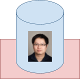
You can see all the 3D features of the cylinder by looking at its side.
Now, peer over and look at the cylinder from an eagle eye view, looking down.

Now it looks like a 2D shape.
So we’ve gone from seeing all 3D features to just seeing 2D features. We’ve gone down by a dimension!
This is called projection and we can use this with data, too.

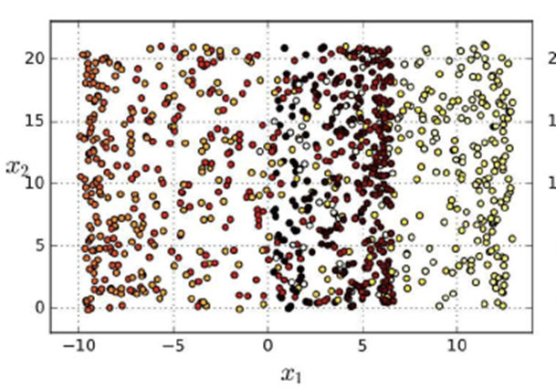
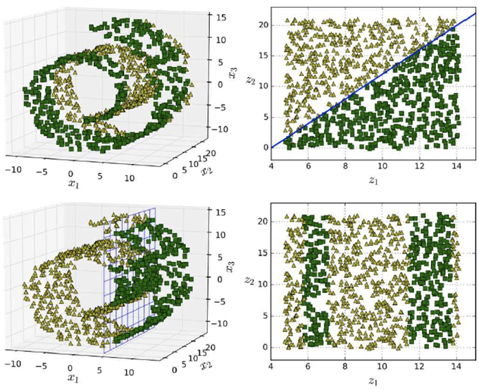
For example, look at this data set:

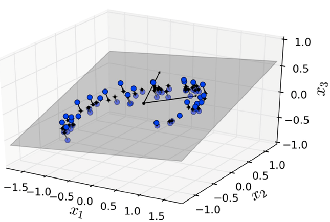
It seems to swirl around, but the x3 axis seems to hold little in the way of correlation.
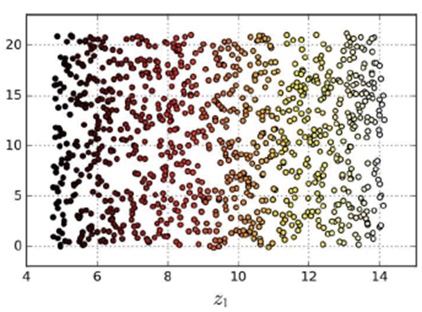
If we just “project”:

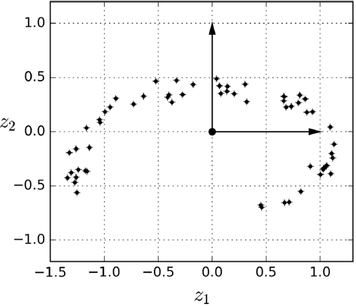
Boom! We get something that looks a little nicer.

Manifold learning

However, projection doesn’t always work. Here’s an example with a Swiss roll data set:

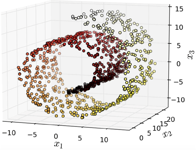
Once you finish drooling, you’ll notice that there’s no angle to “reduce” this with.

Yeah... that doesn’t look very good.

We kind of need to “unravel” or “uncurl” the dataset to get a nice gradient of data points.

So how do we do that?
We use another technique, called manifold learning.

Now, you may ask: what is a manifold?
If you already know, you can skip this part.
Let me ask you a question: is a sheet of paper 2D or 3D?
Sure, it exists in our 3D world and it technically has a thickness of 0.1mm, but it has two faces and is just like a 2D surface.
Let’s reduce the dimensions a bit. What about a circle? Is that 2D, or 1D?
You may be thinking “wtf matt it’s 2d idiot worst notes”
But a circle is just a line that’s been bent to meet two ends. So why can’t we see it as 1D?
This type of thinking serves as the foundation of manifolds!
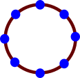
A circle is a 1-dimensional manifold, and I’ll show you why:

It’s 2D, yeah, but what if we were to plot out points all across the circumference and lay it out flat:

Now it’s 1D!
What we’ve done here is we’ve picked a point on this shape, located all the neighbours and mapped the neighbours to a Euclidean space of one dimension (a straight line).
Because we can map this group to a space of one dimension, we call this shape a one-dimensional manifold.
Makes more sense?
Let’s try a less theoretical example and go back to our sheet of paper.

Let’s pick a point on this sheet of paper.

Now we can select a group of neighbours to that point:

Those neighbours can map to a 2D surface (as you can see, it’s a square)!
That makes a sheet of paper a two-dimensional manifold!
Once you understand the concept a bit better, you don’t even have to bother picking a point; you can just sort of tell using intuition.
For example, a torus (or a doughnut):

What n-manifold is that?
Well, the surface area is all 2D, so it’s a 2-dimensional manifold.
You can think of it like “unwrapping” the surface of an object and seeing what the dimensions of that wrapping is.
For example, a circle being “wrapped” by a 1D curved line.
So basically, a manifold is a warped version of a low dimensional shape in a higher dimensional space, for example:

A 1D line warped to make a 2D circle
A 2D surface warped to make a 3D sheet of paper or a 3D doughnut

Hopefully, it makes more sense. The slides did not go into this much detail but I wanted to explain it, because I always used to wonder about the dimensionality of a piece of paper when I was younger.

If we have a dataset, could we “unwrap” that, like in our manifold examples?
Yes, we can!
It doesn’t always work, though, but it works well for data sets like this:

Principal Component Analysis (PCA)

PCA is a projection method.
It’s the most popular dimensionality reduction method.
It identifies the hyperplane that lies closest to the data, and then it projects the data onto it.
The problem is: how do we identify that hyperplane?
I think it’s easier if you just look at an example:

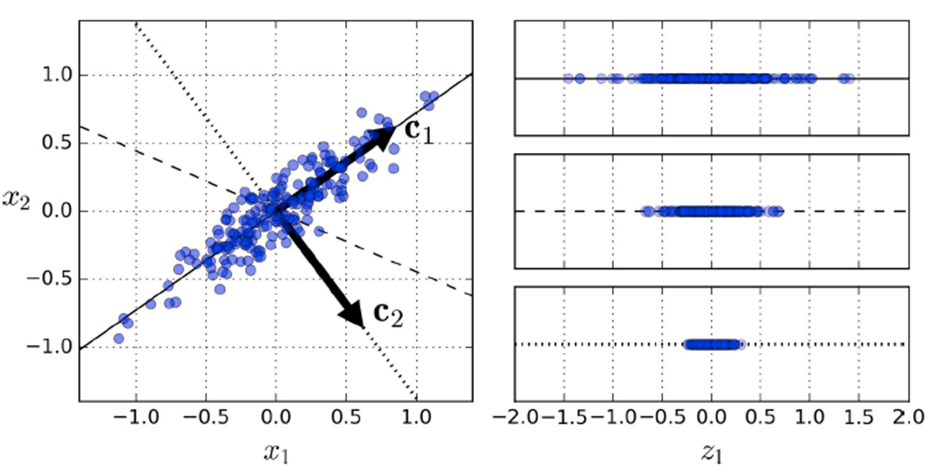
On the right, which vector should we pick to project onto?
The first?
The second?
The third?
The best one is the first because it has the most variance.
That first “dimension” is called the first principal component: the dimension of the data in which the variance is the highest.

The way PCA works is it keeps identifying orthogonal axes, trying to maximise variance, until it reaches the desired number of dimensions.
However, it can only get rid of “useless” dimensions: if there are no useless dimensions, or if all dimensions hold an even amount of information, then PCA won’t work.

Basically, PCA takes correlated variables and projects into uncorrelated variables.

How do we pick the right number of dimensions?
Generally we pick the number of dimensions that add up to a sufficiently large portion of the variance.
For data visualisation, maybe we’d want to reduce it down to 2 or 3 dimensions.

Sometimes, we can’t fit the entire dataset into memory.
For that, we can do incremental PCA by splitting the data into mini-batches.
We can also do randomised PCA to find approximations of the first principal components. It’s much faster than regular PCA.
You can even use that kernel trick thing we saw with kernel PCA, which is used for non-linear datasets.

Locally Linear Embedding (LLE)

Unlike PCA, LLE is a manifold learning technique.
LLE measures how each training instance linearly relates to its closest neighbours.
It then looks for a low-dimensional representation of the training set where these local relationships are best preserved.

So it basically collects the relationships between the data points, and it selects the best dimensional reductions that preserve those relationships the best.

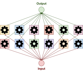
Artificial Neural Nets (Chapter 10)

Neural networks: Bottom-up classification
Neuron:

What it does:

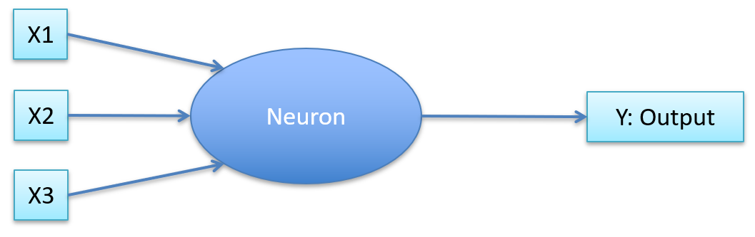
Aggregates inputs
If it’s above a threshold, fire a signal
If not above threshold, do not fire a signal

Perceptron model:

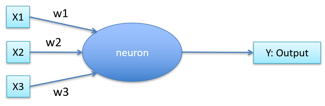
Each input has a weight
It takes the weighted sum
Is put through some aggregate function
If above threshold, fire. If not, don’t fire.
Pretty much the same as before, but it has weights.
It can also self-train.

What’s the aggregate function?
Sum? Not very expressive.
That’s why we have weights; to say which input is more important.
We can also have a “bias”

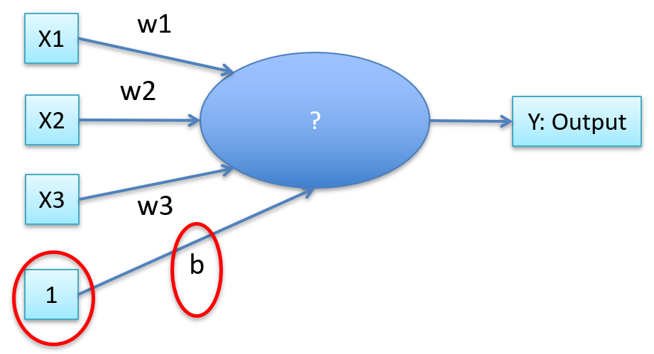
Then our aggregate function is

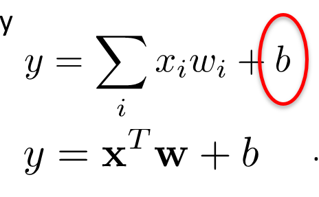
That’s linear regression
Types of activator function:

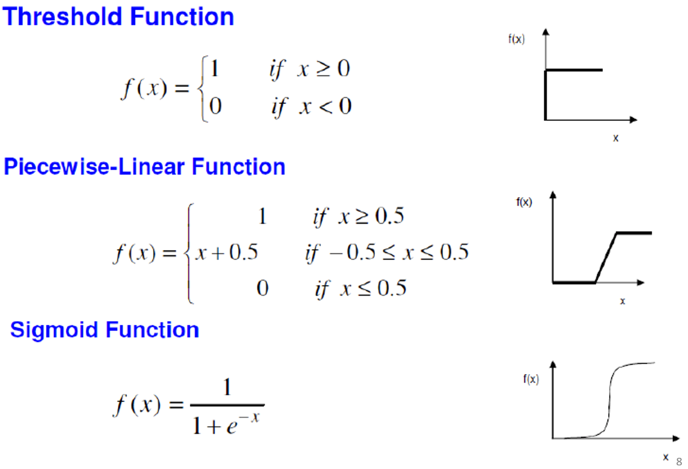
Cannot separate things that are not linear with one neuron
To separate things that are non-linear, we use more than one neuron

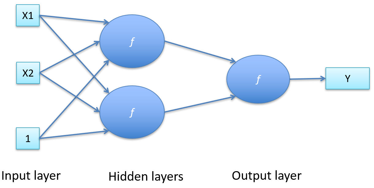
Perceptrons feed into other perceptrons
It’s more “black box”

How do we train the weights?

Could use gradient descent, but that’s only for the last hidden and output layer.
What about the other hidden layers?
We use backpropagation of errors.

Backpropagation method:

Build a loss function L
Employ calculus to calculate partial derivative of L with respect to each weight
Use differentiable activation function (usually sigmoid)
We now know which way we need to “nudge” each weight for a given training sample

This requires a lot of work, though.
However, we now have GPUs and grid computing, so we can do it.

Deep learning: transform input space to higher level abstractions with lower dimensions (similar to feature expansion)

Multi-layer architecture (many hidden layers)
Each layer responsible for space transformation step
Complexity of non-linearity is decreased
Very expensive

Deep Neural Nets (Chapter 11)

Problems with neural nets:

Vanishing gradients

Training = backpropagation
Weight changes only really happen in the last few layers, and changes become negligible in the front layers.
Therefore we’re wasting resources having all those layers at the start.
The gradients from the back layers to the start layers are “vanishing”
Glorot & Bengio (2010) found out it’s because:

we’re using the sigmoid function
random initialisation with “truncated Gaussian” randomness distribution (random initial weights)

Mitigation strategy 1: different random initialisation
OK, so part of the problem is setting up the initial weights. How do we mitigate that?
Xavier initialisation!
Go here if you wish to further understand Xavier initialisation: https://prateekvjoshi.com/2016/03/29/understanding-xavier-initialization-in-deep-neural-networks/

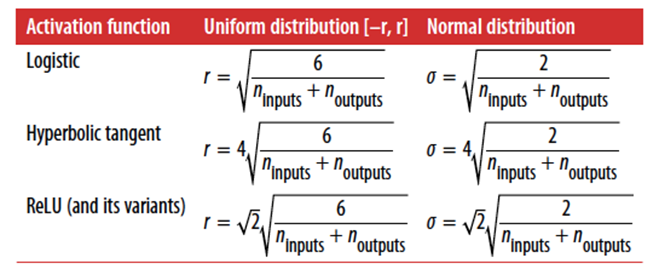
Mitigation strategy 2: different activation functions
Also, part of the problem is using the sigmoid activation function.
To fix that, we use non saturating activation functions:

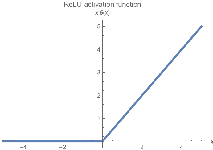
Most popular is ReLU (rectified linear unit)
Easy to compute, no limit on max value
However, neurons can get stuck on a zero gradient and “die”
Half of all neurons can get this

Do you want the neurons to die or do you want the neurons to survive?
Survive, of course!
We can use a variant called Leaky ReLU, where there are no non-zero gradients

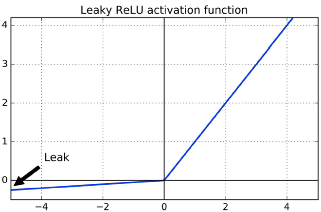
However, we can’t differentiate when x = 0.
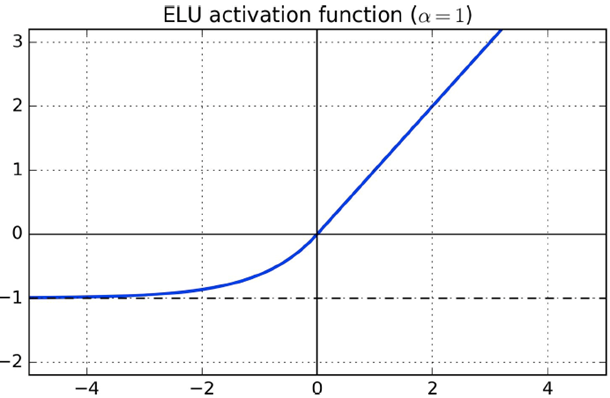
So what can we use?

ELU (exponential linear unit)
It’s smooth everywhere, which is good

Mitigation strategy 3: batch normalisation

It normalises the inputs, centering them around 0
Uses 2 new parameters
It reduces vanishing / exploding gradients, but it’s computationally slow

Exploding gradients

Like vanishing gradients, but instead of the weight updates being negligible, the weight updates get bigger and more unstable until they essentially “explode” into ridiculous weight changes.

Mitigation strategy 1: batch normalisation
Mitigation strategy 2: gradient clipping

Clip gradient if it gets too big
Often used in RNNs

Slow training with gradient descent techniques

Transfer learning: reuse networks already trained on similar problems

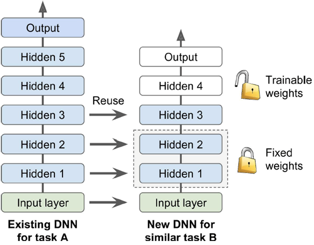
You need to find a “sweet spot” for the number of layers to copy.
It can speed up training of the second model.

Faster optimisers:

Stochastic gradient descent (SGD)
Doesn’t converge to the optimum; it oscillates around it
How do we fix that?
We use:

Momentum optimization
Nesterov Accelerated Gradient
AdaGrad
RMSProp
Adam (adaptive moment estimation)

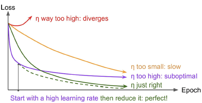
How do we set our learning rate in optimisation algorithms?
We start large, then gradually reduce it

Overfitting issues in large networks

Too many parameters (weights, neurons, layers etc.) makes overfitting more likely
To fix this, we use regularisation.
Early stopping:

Train on a mini-batch, then run on validation set, then train again (on another batch)
But stop training as soon as error rate on validation set starts increasing (performance starts dropping)

Dropout:

What’s a dropout? Is it you after Machine Learning Technologies?
At every training step, every neuron (excluding the output layer) has a probability p of being entirely ignored within that training step
It usually significantly slows down convergence (by a factor of 2), but it’s typically worth the time and effort.
In practice p ~ 0.5
Usually leads to 1-2% accuracy boost

Data augmentation:

Artificially generate new data points from existing ones
Add some noise to existing data but keep the same label

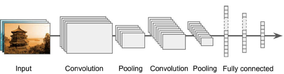
Convolutional Neural Nets (Chapter 13)

Neural networks are the state-of-the-art solution to classification of visual objects
DNNs with fully connected layers (each node is connected to every other node):

Can learn almost any data model
If we don’t need a connection, set the weight close to 0

Issues:

Too many parameters
100x100 picture => 1st hidden layer has 1000 neurons => 10 million connections

How do we fix this?
Give up on full connectivity
Instead have convolutional layers and make a CNN:

Motivated by nature
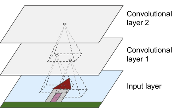
Convolutional layers are not connected to everything, but only pixels in their receptive fields / only neurons in the previous layer
Faster to train
Less sensitive to transformations like translation or rotation

Zero padding:

When shrinking down neurons to a single neuron, we pad zeroes around the neurons on the edges

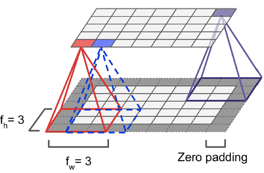
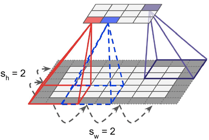
Reducing size of convolutional layer:

Use strides
Strides lets you jump between neighbouring rectangles
Basically, in the picture above, the distance between the red and the blue rectangles is just one pixel.
With strides, the offset is bigger.
Larger strides reduces layer size, but lose information

Filters:

The weight of the edges that connect the rectangle to the new neuron form a matrix
That matrix is the “filter” that decides what information the new neuron will take from the square

Using a variety of filters may abstract the raw input into more expressive data, increasing the accuracy of our models.

Feature map:

Where the whole layer applies the same filter

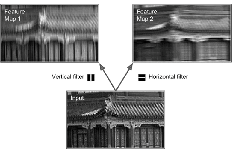
In training, the CNN learns the most useful filters and combines them into more complex patterns

Stacking feature maps:

Packing 2D feature layers on top of each other -> 3D stacks
It’s just a fancy way of saying that we’re applying multiple feature maps for every layer.

Memory requirements:

CNNs need loads of RAM
What to do when it crashes because it runs out of memory?

Reduce mini-batch size
Reduce dimensionality using stride
Use 16-bit floats instead of 32-bit floats
Distribute CNN across multiple devices

Pooling layers:

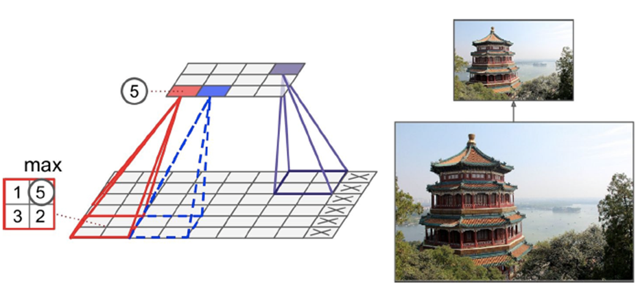
Goal: reduce input image size to reduce computational load
CNN can tolerate small image shift
Pooling layer: a convolutional layer with no weights; it is “stateless”
Performs some kind of aggregation, like max (max pooling) or mean (average pooling)

Famous CNN architectures:

LeNet-5 - Used for handwritten digit recognition
AlexNet - 17% top-5 error rate; stacked convolutional layers on each other instead of pooling
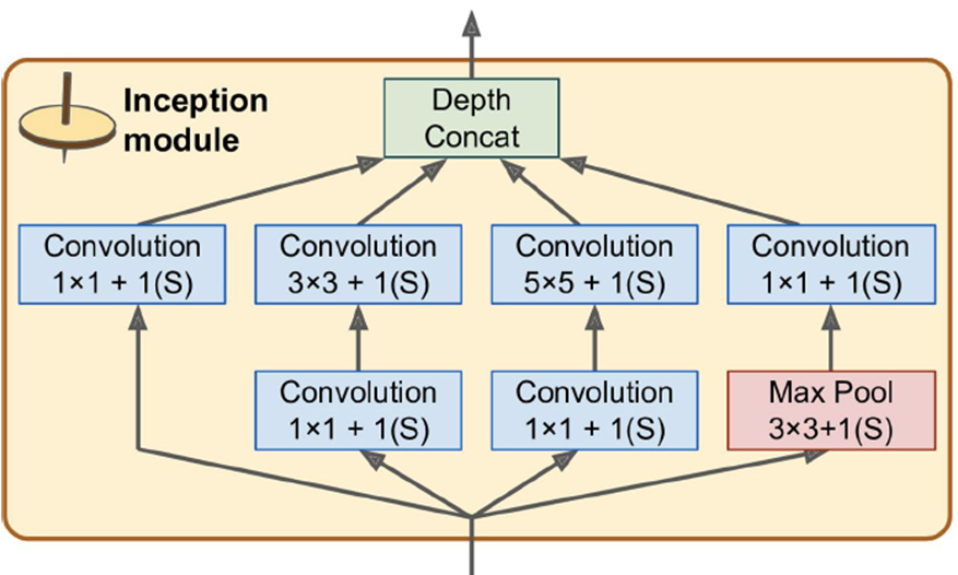
GoogLeNet - 7% top-5 error rate; much deeper and had 10 times fewer params than AlexNet

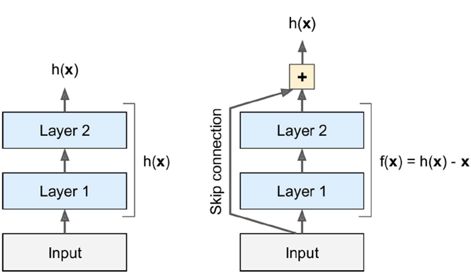
ResNet - 3.6% top-5 error rate; has 152 layers, skips connections (called shortcuts)

Recurrent Neural Nets (Chapter 14)

Normally, with classification and regression, we predict Y for a given X.
What if we want to guess future events?
It usually depends on previous sets of data (historical data)

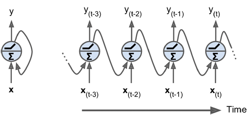
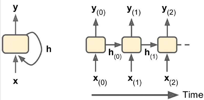
In recurrent neural nets, the output of a neuron feeds into its input
It’s a self-loop.
So over time, the network develops:

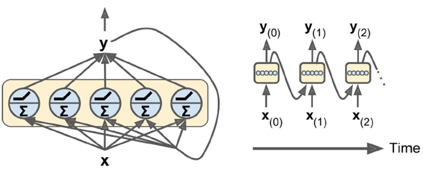
We can make it more complex with a vector of inputs + outputs.
Two weights: one for input x(t) and one for output of previous step y(t - 1)

Memory cells: part of the network can preserve state, so we can store a good partial solution
State of memory cell: h(t) = f(h(t - 1), x(t))

Four types of RNNs:

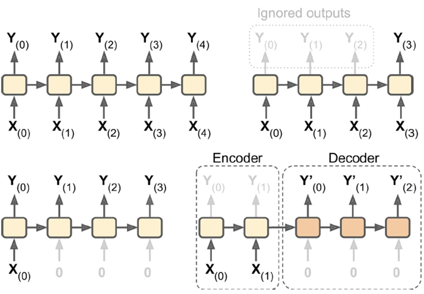
Sequence-to-sequence: feed in a stream of data, receive a stream

E.g. input: video, output: frame-by-frame caption
(still not suitable for visual question and answering)

Sequence-to-vector: feed in a stream of data, receive a single answer

E.g. input: book review, output: sentiment value

Vector-to-sequence: feed in one data point, receive a stream

E.g. input: image, output: image caption

Encoder-Decoder: sequence-to-vector encoder output is passed as input to vector-sequence decoder

E.g. input: sentence in english, output: translated sentence in german

How to train RNNs:

Unroll network through time, use back propagation
Usually network is very large though
Mitigations:

ReLU
Dropout
Gradient clipping, faster optimisers etc.
Truncated backpropagation: set a time horizon for the rolling out

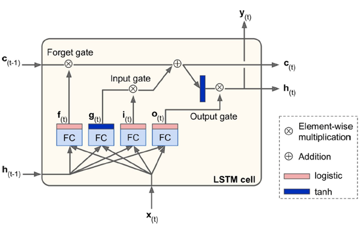
Long Short-Term Memory (LSTM):

2 states: h(t) for short-term, c(t) for long-term
LSTM cells can recognise an important input and store it in long-term state

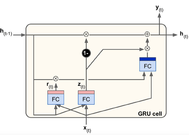
Gate Recurrent Unit (GRU):

Simpler version of LSTM
Performance is still as good as LSTM

Implementation

SVMs

You use the class LinearSVR from the sklearn.svm module for linear SVMs and SVR for non-linear SVMs (from the same module).
For classifiers, just change the R to a C to make LinearSVC and SVC.
You can use a Pipeline to scale the data and do all sorts of operations before feeding it into the SVM regressor.

Linear SVM regression

from sklearn.svm import LinearSVR
from sklearn.pipeline import Pipeline

# Without pipeline
svm_reg = LinearSVR(epsilon=1.5)

# With pipeline
svm_reg = Pipeline((
("scaler", StandardScaler()),
("linear_svc", LinearSVC(
C=1,
loss="hinge")),
))

svm_reg.fit(X, y)

Parameters (LinearSVR)
C		Regularisation parameter. Strength of regularisation is inversely proportional to C.
epsilon		Epsilon parameter for epsilon-insensitive loss function.
loss		Specifies loss function

Non-linear SVM regression

from sklearn.svm import SVR

svm_poly_reg = SVR(
kernel="poly",
degree=2,
C=100,
epsilon=0.1)
svm_poly_reg.fit(X, y)

Parameters (SVR)
C		Regularisation parameter. Strength of regularisation is inversely proportional to C.
epsilon		Epsilon parameter for epsilon-SVR model.
kernel		Specifies kernel type
degree		Degree of polynomial kernel function

Polynomial features

from sklearn.preprocessing import PolynomialFeatures

poly_svm_clf = Pipeline((
("poly_features", PolynomialFeatures(degree=3)),
("scaler", StandardScaler()),
("svm_clf", LinearSVC(

C=10,

loss="hinge"))
))

Parameters

(PolynomialFeatures)

degree

The degree of polynomial features

include_bias

If true, includes a bias column of all ones, where all polynomial powers are zero

Kernel trick

svm_reg = Pipeline((
("scaler", StandardScaler()),
("linear_svc", SVC(
kernel="poly", # Include this
degree=3,
coef0=1,
C=5)),
))

Parameters

(SVC, given that kernel=”poly”)

coef0

Independent term in kernel function

RBF kernel

svm_reg = Pipeline((
("scaler", StandardScaler()),
("linear_svc", SVC(
kernel="rbf",
gamma=5,
C=0.001)),
))

Parameters

(SVC, given that kernel=”rbf”)

gamma

Can be ‘scale’, ‘auto’ or float

Kernel coefficient for ‘rbf’

Decision trees

Just use either DecisionTreeClassifier or DecisionTreeRegressor.

Classification

from sklearn.tree import DecisionTreeClassifier

tree_clf = DecisionTreeClassifier(

max_depth=2)
tree_clf.fit(X, y)

Parameters

(DecisionTreeClassifier)

max_depth

Maximum depth of the tree

criterion

The function to measure the quality of a split.

Can either be “gini” or “entropy”.

Regression

from sklearn.tree import DecisionTreeRegressor

tree_clf = DecisionTreeRegressor(

max_depth=2)
tree_clf.fit(X, y)

Parameters

(DecisionTreeRegressor)

max_depth

Maximum depth of the tree

Ensemble learning

To ensemble multiple classifiers together, use the VotingClassifier class in sklearn.ensemble. For regression, simply use VotingRegressor.

from sklearn.ensemble import RandomForestClassifier
from sklearn.ensemble import VotingClassifier
from sklearn.linear_model import LogisticRegression

log_clf = LogisticRegression()
rnd_clf = RandomForestClassifier()
svm_clf = SVC()

voting_clf = VotingClassifier(
estimators=[
('lr', log_clf),
('rf', rnd_clf),
('svc', svm_clf)
],
voting='hard'
)
voting_clf.fit(X_train, y_train)

Parameters

(VotingClassifier)

estimators

List of classifiers to ensemble

voting

The type of voting, either ‘hard’ or ‘soft’

Bagging and pasting

Scikit-learn uses BaggingClassifier to perform bagging.
It’s like an alternative to VotingClassifier that uses bagging.
Except with BaggingClassifier you need to use the same base estimator for all estimators.

from sklearn.ensemble import BaggingClassifier

bag_clf = BaggingClassifier(
DecisionTreeClassifier(),
n_estimators=500,
max_samples=100,
bootstrap=True,
n_jobs=-1
)
bag_clf.fit(X_train, y_train)
y_pred = bag_clf.predict(X_test)

Parameters (BaggingClassifier)
base_estimator		The base estimator to fit on random subsets of the dataset
n_estimators		The number of base estimators in the ensemble
max_samples		The number of samples to draw from X to train
bootstrap		If true, bagging (with replacement) If false, pasting (without replacement)
n_jobs		The number of jobs to run in parallel. -1 means using all processors.

Random forest

You can either use a BaggingClassifier with DecisionTreeClassifiers, or just use a RandomForestClassifier.

# Code v1: optimised for decision trees
from sklearn.ensemble import RandomForestClassifier

rnd_clf = RandomForestClassifier(
n_estimators=500,
max_leaf_nodes=16,
n_jobs=-1)
rnd_clf.fit(X_train, y_train)

# Code v2: generic solution
bag_clf = BaggingClassifier(
DecisionTreeClassifier(
splitter="random",
max_leaf_nodes=16),
n_estimators=500,
max_samples=1.0,
bootstrap=True,
n_jobs=-1
)

Parameters (RandomForestClassifier)
n_estimators		The number of trees in the forest
max_leaf_nodes		Grow trees with max_leaf_nodes in best-first fashion
n_jobs		The number of jobs to run in parallel. -1 means using all processors.

Gradient boosting

# Code v1: Manual
from sklearn.tree import DecisionTreeRegressor

tree_reg1 = DecisionTreeRegressor(max_depth=2)
tree_reg1.fit(X, y)

# Next predictor
y2 = y - tree_reg1.predict(X)
tree_reg2 = DecisionTreeRegressor(max_depth=2)
tree_reg2.fit(X, y2)

# Next predictor
y3 = y2 - tree_reg1.predict(X)
tree_reg3 = DecisionTreeRegressor(max_depth=2)
tree_reg3.fit(X, y3)

# Prediction
y_pred = sum(tree.predict(X_new) for tree in (tree_reg1, tree_reg2, tree_reg3))

# Code v2: Automatic
from sklearn.ensemble import GradientBoostingRegressor

gbrt = GradientBoostingRegressor(
max_depth=2,
n_estimators=3,
learning_rate=1.0)
gbrt.fit(X, y)

Parameters (GradientBoostingRegressor)
max_depth		Maximum depth of the individual regressors
n_estimators		Number of boosting stages to perform
learning_rate		Shrinks the contribution of each tree by learning_rate

Dimensionality reduction

Principal Component Analysis (PCA)

from sklearn.decomposition import PCA

# Explicitly state number of dimensions
pca = PCA(n_components=2)

# Choose no. of dimensions that add up to
# sufficiently large portion of variance
# (in this case, 95%)
pca = PCA(n_components=0.95)

X2D = pca.fit_transform(X)

Parameters

(GradientBoostingRegressor)

n_components

Number of components to keep

Incremental PCA

from sklearn.decomposition import IncrementalPCA

n_batches = 100
inc_pca = IncrementalPCA(n_components=154)

# Splits batches called X_batch and fits them
for X_batch in np.array_split(X_mnist, n_batches):
inc_pca.partial_fit(X_batch)

# Performs transformations at once
x_mnist_reduced = inc_pca.transform(X_mnist)

Parameters

(GradientBoostingRegressor)

n_components

Number of components to keep

Kernel PCA

from sklearn.decomposition import KernelPCA

rbf_pca = KernelPCA(
n_components=2,
kernel="rbf",
gamma=0.04)
X_reduced = rbf_pca.fit_transform(X)

Parameters (GradientBoostingRegressor)
n_components		Number of components to keep
kernel		Type of kernel
gamma		Kernel coefficient

Locally Linear Embedding (LLE)

from sklearn.decomposition import LocallyLinearEmbedding

lle = LocallyLinearEmbedding(
n_components=2,
n_neighbours=10)
X_reduced = lle.fit_transform(X)

Parameters

(GradientBoostingRegressor)

n_components

Number of coordinates for the manifold

n_neighbours

Number of neighbours to consider for each point

Deep Neural Nets

From now on we’re using Tensorflow

Setting up

import tensorflow as tf

n_inputs = 28 * 28 # MNIST
n_hidden1 = 300
n_hidden2 = 100
n_outputs = 10

X = tf.placeholder(tf.float32, shape=(None, n_inputs), name="X")
y = tf.placeholder(tf.int64, shape=(None), name="y")

Setting up a layer

def neuron_layer(X, n_neurons, name, activation=None):
with tf.name_scope(name):
n_inputs = int(X.get_shape()[1])
stddev = 2 / np.sqrt(n_inputs)
init = tf.truncated_normal((n_inputs, n_neurons), stddev=stddev)
W = tf.Variable(init, name="weights")
b = tf.Variable(tf.zeros([n_neurons]), name="biases")
z = tf.matmul(X, W) + b
if activation == "relu":
return tf.nn.relu(z)
else:
return z

Setting up a full DNN

with tf.name_scope("dnn"):
hidden1 = neuron_layer(X, n_hidden1, "hidden1", activation="relu")
hidden2 = neuron_layer(hidden1, n_hidden2, "hidden2", activation="relu")
logits = neuron_layer(hidden2, n_outputs, "outputs")

Setting up the loss function

with tf.name_scope("loss"):
xentropy = tf.nn.sparse_softmax_cross_entropy_with_logits(labels=y, logits=logits)
loss = tf.reduce_mean(xentropy, name="loss")

Setting up the training part

learning_rate = 0.01
with tf.name_scope("train"):
optimizer = tf.train.GradientDescentOptimizer(learning_rate)
training_op = optimizer.minimize(loss)

Evaluating performance of model

with tf.name_scope("eval"):
correct = tf.nn.in_top_k(logits, y, 1)
accuracy = tf.reduce_mean(tf.cast(correct, tf.float32))

Initialise model parameters

init = tf.global_variables_initializer()
saver = tf.train.Saver()

Full training code for DNNs

with tf.Session() as sess:
init.run()
for epoch in range(n_epochs):
for iteration in range(mnist.train.num_examples // batch_size):
X_batch, y_batch = mnist.train.next_batch(batch_size)
sess.run(training_op, feed_dict={X: X_batch, y: y_batch})
acc_train = accuracy.eval(feed_dict={X: X_batch, y: y_batch})
acc_test = accuracy.eval(feed_dict={X: mnist.test.images, y: mnist.test.labels})

print(epoch, "Train accuracy:", acc_train, "Test accuracy:", acc_test)

save_path = saver.save(sess, "./my_model_final.ckpt")

Using DNNs

with tf.Session() as sess:
saver.restore(sess, "./my_model_final.ckpt")
X_new_scaled = [...] # some new images (scaled from 0 to 1)
Z = logits.eval(feed_dict={X: X_new_scaled})
y_pred = np.argmax(Z, axis=1)

Convolutional Neural Nets

Stacking feature maps

import numpy as np
from sklearn.datasets import load_sample_images

# Load sample images
dataset = np.array(load_sample_images().images, dtype=np.float32)
batch_size, height, width, channels = dataset.shape

# Create 2 filters
filters_test = np.zeros(shape=(7, 7, channels, 2), dtype=np.float32)
filters_test[:, 3, :, 0] = 1 # Vertical line
filters_test[3, :, :, 1] = 1 # Horizontal line

# Create a graph with input X plus a convolutional layer applying 2 filters
X = tf.placeholder(tf.float32, shape=(None, height, width, channels))
convolution = tf.nn.conv2d(X, filters, strides=[1,2,2,1], padding="SAME")

with tf.Session() as sess:
output = sess.run(convolution, feed_dict={X: dataset})

plt.imshow(output[0, :, :, 1]) # Plot 1st image's 2nd feature map
plt.show()

X	input mini-batch (4D tensor)
filters	set of filters to apply (also 4D tensor)
strides	4 element 1D array two central elements are the vertical and horizontal strides. The first and last elements must currently be equal to 1 (They may one day be used to specify a batch stride - to skip some instances, and a channel stride - to skip some of the previous layer’s feature maps or channels)
padding	must be “VALID” or “SAME”

Pooling layers

[...] # load the image dataset, just like above

# Create a graph with input X plus a max pooling layer
X = tf.placeholder(tf.float32, shape=(None, height, width, channels))
max_pool = tf.nn.max_pool(X, ksize=[1,2,2,1], strides[1,2,2,1], padding="VALID")

with tf.Session() as sess:
output = sess.run(max_pool, feed_dict={X: dataset})

plt.imshow(output[0].astype(np.uint8)) # plot the output for the 1st image
plt.show()

Recurrent Neural Nets

X = tf.placeholder(tf.float32, [None, n_steps, n_inputs])

basic_cell = tf.contrib.rnn.BasicRNNCell(num_units=n_neurons)
outputs, states = tf.nn.dynamic_rnn(basic_cell, X, dtype=tf.float32)

TL;DR

Welcome back to the TL;DR section, where we summarise everything above!

Huh? Where is everything?

I’m doing things a little differently for this module.
Call it an “experiment” if you will.
For this module, the TL;DR section will be a TL;DR document.
This’ll hopefully reduce lag (like in the Engineering Management and Law doc)
However, it’ll split up the comments and suggestions into two documents, which is a downside to having separate documents.

If this proves to have more pros than cons, I’ll keep doing this in the future.
Click here to go to the TL;DR document!

Note: The TL;DR document will not include a summary of the implementation section.

Practical Use Cases

Here’s some notes about Stuart’s lectures.
I don’t think this’ll come up in the exam, so they’re unfinished for now.

Introduction to practical use cases

Textbook ‘idealised’ workflow:

Problem: Look at the big picture
Data: Get the data
Data, Algorithm Design: Discover and visualise to gain insights
Algorithm Design: Prepare the data for machine learning algorithms
Algorithm Design & Implementation: Select a model and train it
Evaluation, Iteration: Fine-tune your model
Release: Present your solution
Maintain: Launch, monitor and maintain your system

Practical iterative workflow (for addressing any problem):

Problem characterization

Objectives
Success metrics
Availability of data
Customer constraints
Flexibility

Data characterization

Representation
Ground truth
Volume / throughput (how much data)
Quality (not all data is clean)
Bias
Legal & ethics (privacy)

Data analysis & hypothesis formulation

Visualise
Identify patterns & correlations
Natural classes & clusters
Form hypotheses for algorithm choices

Algorithm choices

Pre-processing
Feature selection + extraction
Dimensionality reduction
Machine learning algorithm
Algorithm attributes need to suit problem and data characteristics

Algorithm implementation
Evaluation setup & analysis

Visualise results
Confusion matrix
Fault analysis
Under / Overfitting
Causal analysis
Statistical significance

Iterative improvement

Improve feature selection
Explore parameter space
Get more training data
Parallelize
Test alternative algorithm designs

Release
Maintain

Deliverables and Deadlines:

Machine learning algorithm implementation

COMP 3222 - UG, Week 9 [Friday 29th Nov 2019]
Marking weight 0%
3 Top performing algorithms enter 'hall of fame' (no impact on marks) TurnItIn checked

Final report

COMP 3222 - UG , Week 9 [Friday 29th Nov 2019]
COMP 6246 - MSc , Week 9 [Friday 29th Nov 2019]
Marking weight 50%

Feedback

Week 12 [Friday 20th Dec 2019]

Coursework intro

Task and Data

Task: Design an algorithm to spot fake news from posts with images or videos
What’s fake news?

Reposts in a different context
Edited video / images
Artwork / snapshots presented as real imagery

Dataset:

It’s a zip file on the module page
There’s 3,781 test posts
There’s 14,483 training posts
No training on the test data (that’s cheating)
Each post contains text and embedded image / video
It’ll come as a CSV with these columns:

Tweet ID
Tweet text
User ID
Image ID(s)
Username
Timestamp
Label

NO PROCESSING IMAGES
Only process text and metadata

Design and Implementation

Go through the process that we’ve gone through before
There’s more emphasis on reaching the algorithm and the process than the actual algorithm itself

Do it in Python
Use Scikit-Learn and / or TensorFlow
You can use other Python libraries if you want
Report F1 scores for each algorithm test in final report
Submission should include instructions on how to install, run and generate F1 scores
Submit to C-BASS system