Computing costs less
We can introduce processing power into places and devices that would’ve otherwise been uneconomic
Edge computing: data is processed at the edge of the network (real-time “instant data” generated by sensors or users)

Interconnection

Computers are networked into distributed systems
They can talk to each other and help each other

Intelligence

Computers are smart (sort of)
They can complete really complex tasks, like making a move in chess, or deciding if a picture has a cat in it or not.

Delegation

We are passing down more and more tasks to computers.
We’re giving control to them, even for safety-critical tasks, such as aircrafts and self-driving cars.

Human-orientation

Computers are meant to augment human intelligence.
They’re meant to do stuff for us.
That means they need input from us, such as decision preferences.

So what?
Well, each of these trends imply that:

Computers need to act independently
Computers need to represent our best interest
Computers need to cooperate, reach agreements or even compete.

Together, they’ve led to the emergence of a new field:

Wow! Lots of agents working together in a system!
... what’s an agent?

Agents

An agent is:

“A computer system capable of autonomous action in some environment, in order to achieve its delegated goals”

In layman’s terms, an agent is a computer system that lives in some kind of changing environment, and it performs automatic actions to try and achieve a goal defined by us: the human overlords.
The key points are:

Autonomy: capable of independent action without need for constant intervention (can do stuff by itself)
Delegation: acts on behalf of its user or owner (represents our best interests)

We think of an agent as being in a close-coupled, continual interaction with its environment:

sense → decide → act → sense → decide → ...

An agent:

Perceives the environment through sensors (cameras, TCP/UDP socket, keyboard etc.)
Acts on the environment through actuators (variables, web pages, databases, robotic arms etc.)

Here’s a simple example of an agent: a thermostat.

Delegated goal: maintain room temperature
Perception: heat sensor
Action: switch heat on / off if room temp. is too cold / hot
Input: the heat threshold at which the heat should be turned on at

A pretty plain-looking thermostat. It doesn’t even have RGB.

This one’s a bit boring because the decision is easy: it’s just checking the room temperature against a given threshold.

How do we define an agent that’s a bit... smarter?

Intelligent Agents

An intelligent agent has three behavioural properties:

Reactive

The agent maintains an ongoing interaction with its environment, and responds to change that occurs in it.
Basically, the agent needs to be able to respond to change.

Proactive

The agent needs to generate and attempt to achieve goals and not be driven solely by reacting to events; it needs to take the initiative.
In other words, the agent needs to actually do stuff by itself to achieve its goals and not just react to things that change.
This also includes recognising opportunities, and taking them.

Social

The agent needs the ability to interact with other agents and (usually) humans via cooperation, coordination and negotiation.
Simply, the agent needs to be able to talk to other agents.

There are other properties, such as:

Rationality

Tries to maximise its performance measure with all possible actions.

Learning / Adaptation

Agent improves performance over time

Intelligent Agent Challenges:

How to represent goals and user preferences
How to optimise the decision making
How to learn and adapt and improve over time

Multi-Agent System (MAS)

A multi-agent system (MAS) is one that consists of a number of agents, which interact.

A multi-agent system of smol robots.

Generally, agents act on behalf of users.
They each have different goals and motivations with each other.
Despite that, they all work together to achieve a common goal, like humans (or not; depends on your group assignment)

There are some problems that arises with a MAS:

If it’s every-agent-for-themselves, how do they cooperate?
How can conflicts be resolved, and how can they (nevertheless) reach agreement?
How can autonomous agents coordinate their activities so as to cooperatively achieve goals?

Collaborative MAS:

Agents owned by the same person / organisation
Can be controlled and made to coordinate
More robust than “centralised” system
No incentive needed, as all agents are controlled by the same thing

Self-interested MAS:

Each agent works on behalf of someone else
Each agent is different
“Every agent for themselves”
Still need to cooperate, but needs mechanisms to resolve conflicts

Link with other disciplines:

Robotics
Complex Systems Science
Economics
Philosophy
Game Theory
Logic
Social Sciences

This can be a strength:

Infusing well-founded methodologies into the field

... or a weakness:

There are many different views as to what the field is about

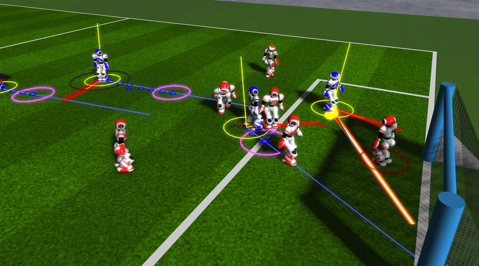
You could even teach a bunch of robot agents to play football with each other.

Classical AI focuses on:

Algorithms to solve hard decision problems; e.g. planning
Algorithms to interpret complex data; e.g. Machine Learning and Machine Vision (I know that’s not classical AI but whatever)
Knowledge representation and reasoning

Agents combine techniques:

Robotics: vision + planning
Software assistants: machine learning + scheduling
E-Commerce ‘bots’: search + machine learning

There are applications of agents:

As a paradigm for software engineering
As a tool for understanding human societies

Agent-Based Negotiation

Part 1

When agents work with each other, there can be conflict.
Conflict is when there is a clash between agents’ different preferences or aims.
This can happen with people, too:

Who’s going to do the washing up?
Where do we go out for dinner?

Conflicts happen in multi-agent systems when:

Agents are self-interested (maximise their own benefit)
Agents represent different stakeholders (different sets of interests / aims)

For example:

A buyer wants to pay as little as possible
The seller wants to sell as much as possible

This is a conflict; the buyer wants to reduce the price, and the seller wants to increase it.

Conflict resolution is possible when there is a mutual benefit to reach an agreement.
In other words, it’s better to reach an agreement than to call the whole thing off.
There’s different types of conflict resolution:

Auctions
Voting
Negotiation

These different types are suited for different situations.

Auctions are used to allocate scarce resources or tasks, such as:

Items to buyers
Advertising space to advertisers
Cloud computing
Tasks to robots
Stocks and shares

To enable auctioning within agents, you must

3D-print a small gavel for them to use.

Auctions are characterised by:

Clearly defined protocol (rules or mechanism) e.g. English auction, Dutch auction, Vickrey auction
Typically requires trusted third party (e.g. auctioneer)
Involves continuous resource such as money
Exploits competition between agents (works well with lots of agents)

Voting is used for group based decisions, called social choices.
Examples:

Where to go out to dinner
Where to build new bridge / services / housing
Which is the best JoJo part

Voting: a core component of a civilised society,

according to Lord of the Flies.

Voting is characterised by:

A single decision from a (typically finite) number of options
Each agent can have different preferences for each option, which is given by a preference order (a.k.a ordinal utility function)
Clearly defined protocol

Negotiation (a.k.a Bargaining) is governed by a protocol which defines the “rules of encounter” between agents, including:

Type of communication allowed
Type of proposals that are allowed
Who can make what proposal at what time

Basically, in a negotiation, different kinds of proposals are made at certain times.
Usually, proposals are made until an agreement is reached or the agents are too stubborn and quit.
The way it works depends on the kind of negotiation protocol we’re using.

An illustration of a negotiation;

not to be confused with TCP/IP.

Negotiations are more flexible compared to other approaches:

You can exchange offers / proposals, but you can also exchange other information such as arguments (reasons why)
Allows for less structured protocols
Often bilateral (between two agents) but can also support multi-party negotiation (more than two agents)

Enables more complex types of agreements (e.g. multi-issue negotiation)
Often decentralised (can involve a mediator)

In case you haven’t noticed, this topic is called Agent-Based Negotiation.
Therefore, we’ll focus on negotiation protocols.

Negotiations are characterised by:

Negotiation environment

Single-issue negotiation (distributive bargaining): e.g. haggling prices. Competitive setting, short-term
Multi-issue negotiation (integrative bargaining): include more issues, allows for mutual benefit and cooperation, long-term

Agent preferences

The preference over possible agreements.
Basically, how “picky” an agent is given an offer.
Specified using utility functions.

Agent negotiation strategies

How the agent behaves.
Defined by the actions taken by the agent at each possible decision point, given information available

Before we move on to the negotiation protocols, it’s worth modelling a single-issue negotiation:

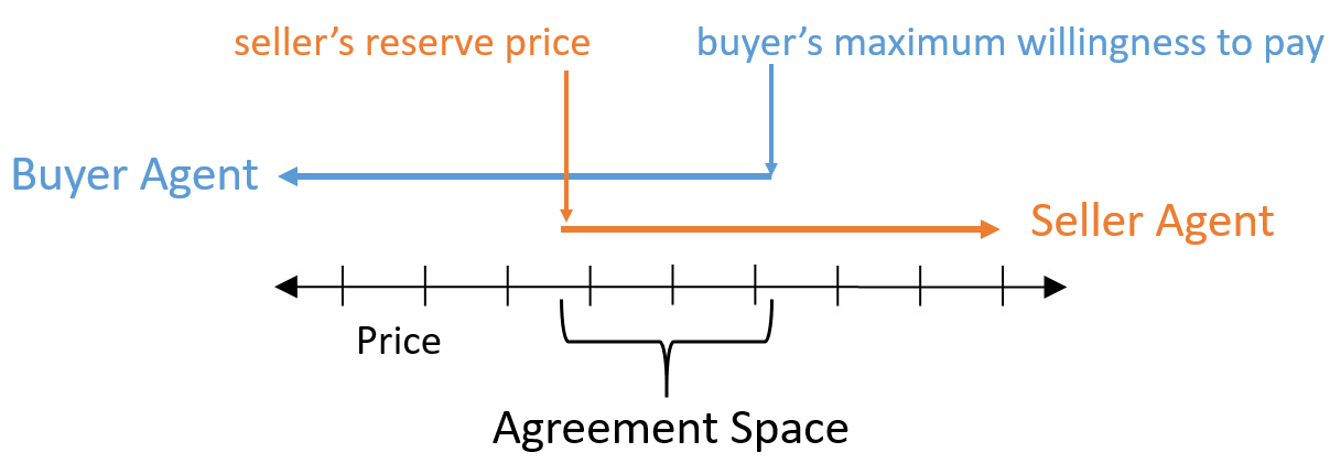
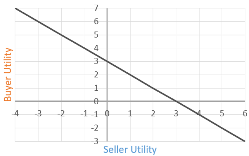
This graph represents a buyer/seller negotiation, and the bottom axis represents the argued price.
The blue arrow is the range of prices the buyer is willing to purchase at, and the orange arrow is the range of prices the seller is willing to sell their product for.
The range of prices at which the buyer and seller arrows intersect is called the agreement space.
That’s the range of prices that both agents are willing to settle for.
The whole point of a negotiation is to scope out the agreement space, but the agents also want to make offers that maximise their aims, e.g. the buyer would want a deal on the far left of the agreement space.

Ultimatum Game

Let’s say you have a cake and need to split it between two agents.
In the Ultimatum Game:

Agent 1 suggests a division of the cake
Agent 2 can choose to accept or reject the cake
If agent 2 rejects, nobody gets the cake

This is also known at the take it or leave it game.

Agent 1 is not a very reasonable agent.

If agent 1 splits the cake in half, it seems fair.
But what if agent 1 leaves agent 2 with a small slither of cake?
Either agent 2 has to accept the tiny slither, or get nothing.
Does that seem fair?

This is called the first-mover advantage.
It means whoever makes the first offer has a significant advantage in the negotiation.

The Ultimatum Game assumes that the agreement space is already known between the agents (the seller’s reserve and buyer’s willingness to pay are shared knowledge).
There’s also no ability to explore the negotiation space, which isn’t so important in this example, but is important when there’s multiple issues.

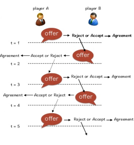
Alternating Offers

The alternating offers protocol consists of a number of rounds, in which offers are exchanged in an alternating fashion.

Agent 1 starts off with an offer.
Agent 2 can accept or reject. If agent 2 rejects, agent 2 can make a counter-offer.
Agent 1 can accept or reject the counter-offer. If agent 1 rejects, agent 1 can make a counter-counter-offer.
This keeps on looping until an agreement is made.

The loop can also end after a deadline of a set number of rounds.

How can they negotiate how much cake to eat

if they don’t have hands to eat with?

A good example is the haggling scene from JoJo.

The vendor suggests ¥1,000 for five kebabs.
Joseph makes a counter-offer of ¥250.
The vendor makes a counter-counter-offer for ¥700.
They converge with the offers ¥300, then ¥600, then ¥350, then ¥550, then ¥400, then ¥450, until eventually they reach a consensus with ¥425.

This is better, but is there any reason for an agent to concede (change their previous offer)?
The vendor could’ve just kept saying ¥1,000, no matter what Joseph said, and created an Ultimatum Game situation.
True, if the vendor kept prices high, Joseph could’ve just walked away.
But in the context of agents, a rational agent will always accept in an ultimatum game.
There needs to be some way to incentivise a concession...

Monotonic Concession Protocol

In the Monotonic Concession Protocol, negotiations proceed in rounds as well, except agents simultaneously propose offers at the same time (without seeing the other offer).

If an agent makes an offer that the other agent rates at least as high as their own offer, an agreement can be made (if both offers are agreeable, one is picked at random).
If not, another round begins.
In the next round, at least one of the agents needs to concede (change their offer).
If neither agent concedes, the negotiation ends without a deal.

What was that? You want an example? The slides are too incompetent to provide a proper explanation?

Buyer	Seller	Description
£5	£30	The buyer wants to buy something, and the seller is selling it at a haggled price. The buyer makes an offer for £5, and the seller makes an offer for £30. These are shown simultaneously. The buyer thinks their offer of £5 is way better for them than the seller’s deal of £30. The seller thinks their offer of £30 is way better for them than the buyer’s deal of £5. Therefore, another round begins.
£10	£20	Both agents concede and make new offers. The prices converge. The buyer still thinks their offer is better off for them than the seller’s offer, and vice versa. Another round!
£10 🐐	£20	The seller does not concede and sticks with the same offer they had before. They’re certain that their product is worth £20 at the least. The buyer is still making an offer of £10, but is also throwing in their best goat into the deal. The seller thinks. Yesterday, at the market, the cheapest goat went for about £12. That means the buyer is basically paying £22, with the value of the goat included. That’s even more than the seller is offering! Right now, the seller is rating the buyer’s offer as greater than or equal to the rating of the seller’s own offer. That means an agreement can be made. The seller walks away with £10 and a new goat, and the buyer walks away with whatever it was the seller was selling (use your imagination).

Source

Divide and Choose

The Divide and Choose protocol is pretty self-explanatory:

Agent 1 divides a continuous resource into partitions.
Agent 2 chooses one of the splitted partitions.

So in the Ultimatum Game example, even if agent 1 partitioned a slither of cake for agent 2, agent 2 could just pick the larger partition, leaving agent 1 with the slither.

Mmmm, cake 🍰

Because the other agent is gonna pick the best slice, agent 1 would want to slice the cake equally, to maximise how much they’ll get.
Therefore every agent will get an equal partition in divide and choose.
This protocol only works for resource allocation problems, where some continuous resource needs to be divided between multiple agents (like cake).

It also works for non-homogenous resources, like if parts of the cake are more attractive (like the candy corn on top of that cake picture above), or in the case of land division.

There’s equivalent protocols that handle more than 2 agents, but it gets complicated.

All in all, the desirable properties of a negotiation are:

Individual rationality: A deal should be better than no deal for all agents
Pareto efficiency: There should be “no money” (or cake) left on the table
The agreement should be “fair”

Part 2

In this part, we’re going to define these concepts more formally.
So I hope you’re fluent in maths syntax.

Utility functions

First of all, we’ll define the utility function.
It is used to model an agent’s preference given an offer.
In other words, this function tells us how much an agent likes an offer.

The utility function is defined as:

Given:

where is the set of all possible offers

This function returns how much the agent likes that offer.

There are two kinds of utility functions:

Ordinal preferences: a preference order is defined, but there is no numerical utility

In other words, we can say and declare that is more preferable than , but that’s it.

Cardinal preferences: each outcome has a numerical utility value

For example, we could say that and
We can always infer ordinal preferences from cardinal ones

Here’s a good example:

A buyer and seller negotiate.
The set of possible outcomes are the price, denoted by , or a disagreement.
The cardinal utility functions are given by:

Where:

is the minimum price the seller is willing to sell for (reserve)
is the maximum price the buyer is willing to buy for (value)

Here, the buyer will prefer to pay less, and the seller will prefer to pay more.
When goes up, will go up and will go down, and vice versa if goes down.
If the price goes below the minimum selling price or above the willing buying price , the seller / buyer will prefer a disagreement, as or will dip below zero.

Utility space

We can visualise this using a utility space.
A utility space is a graph that maps one utility function on one axis, and another utility function on the other.
It allows you to easily see the agreement space given a negotiation.
If that makes no sense, don’t fear: here’s an example.

Given the buyer / seller example above, let’s say and .

We can map the seller utility as the x axis and the buyer utility as the y axis.
Then, we can plot points for all seller / buyer utility values, for all values of .
This will form a line:

For every point on that line, there is a value of that, when plugged in to the utility functions of the seller and buyer, results in the values of the x and y coordinate (a.k.a the utility values of that point on the line).
For example, say we picked the point (1, 2) on the line. That means there is a value of where the seller’s utility is 1, and the buyer’s utility is 2 (spoilers: it’s 5).

What can we do with this graph?
Well, each agent will accept a deal if their utility value is over zero (because if it’s under zero, they’d rather not make a deal).
That means both agents will accept prices if both their utility values are over zero.
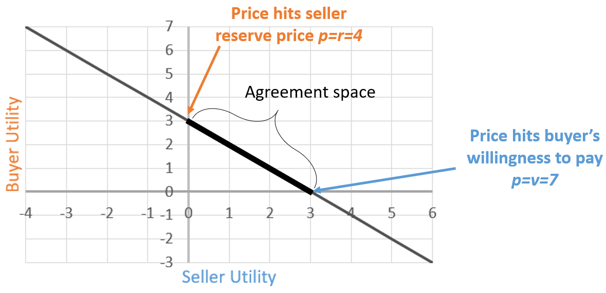
We can find that range by looking at the graph:

Beyond the point (0,3), the price exceeds how much the seller is willing to sell for.
Beyond the point (3,0), the price subceeds how much the buyer is willing to buy for.
That means the line segment between those two points is the sweet spot, or the “agreement space”, at which both agents will be happy.
That also means any value of within that line segment will make those two agents happy.
The agreement space is

We can’t negotiate forever.
We probably have better things to do than spending all night arguing.
There’s different ways to model time pressure:

Deadlines

You must finish the negotiation after a set number of rounds.
Imposed by the protocol (Ultimatum game can only be 1 round long)
Can also be determined by individual constraints

Break-off probability

There’s always a chance that the negotiation will end in any round.
With monotonic concession, if agents don’t concede, everything ends anyway.

Bargaining costs

Costs are applied to the utility functions that grow each round.

Here’s two ways you can model bargaining costs:

Fixed costs:

Like the name says, a fixed cost is applied to the utility function each round.
The cost grows linearly as rounds progress.
More formally, let denote the costs for agent , and is time or bargaining round, then the utility at time is given by:

Discount factors:

After each round, the utility function is shrinked by multiplying it by a number between 0 and 1.
An analogy for this is a melting ice cake; the longer you wait, the more the cake shrinks.
More formally, let be the discount factor of agent , then the utility is given by:

Is it worth putting icing on an ice cake?

This all assumes that we have only one issue: one cake to split, one price to negotiate over etc.
But what if we have many issues to take into account, like time, quality of service, delivery time etc.?
In that case, we can make our offers into vectors, so it would be for each issue .

We can use a weighted additive utility function to calculate a utility value given an offer vector:

That sum looks scary, but don’t worry; it’s just a sum of the utility values of all the issues in the offer vector, but some of them have weights applied to them, so one issue could be more important than another to an agent.

Let’s see an example.
Let’s say we have two cakes: one strawberry and one, uh... chilli flavoured.

I just wanted to be different.

These two cakes represent our two “issues”.
Offer represents the share that agent 1 receives for cake .
This means agent 2 will get .
Agent 1 prefers the strawberry cake, and agent 2 prefers the chilli cake.
The weights will be 7 for a preferred cake and 3 for the other cake.
This results in the utility functions:

What are we waiting for? Let’s see the utility space for this!

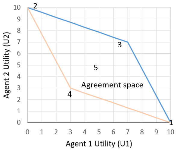
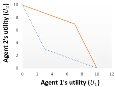
The slides and online lecture go into a bit more detail, but basically:

Point (7,7) is when both agents get all of their preferred cake
Point (5,5) is when both agents get half of both cakes
Point (3,3) is when both agents get all of their non-preferred cake
Point (10,0) is when agent 1 gets both cakes
Point (0,10) is when agent 2 gets both cakes

Within this kite shape are all the possible agreements for this negotiation.

It’s kind of clear that point (7,7) sounds like the best offer, but hear me out: there’s more to it.
Did you notice that the top right half of the kite perimeter is blue?
All the offers within that blue segment are all Pareto efficient.
That means that there’s no further improvement to that offer without making one of the other agents worse off.
The Pareto efficient frontier is the set of all Pareto efficient agreements; in other words, the blue segment.

Basically, there’s no reason not to accept on a Pareto efficient offer.
If you have an offer that is not Pareto efficient, there must be some way to make that offer better for everyone.

There’s even more properties we desire from an offer.
Here’s three of the main ones:

Should be individually rational ( > )
Should be Pareto efficient
Should be fair

Wait, “fair”?
What does fair mean?

Fairness

Fairness is an extra condition for an agreement that makes it more desirable than the others.
Here’s four of them:

Utilitarian social welfare: maximise the sum of utilities

Pick the offer that maximises the sum of all the utility values.
Formally:

Egalitarian social welfare: maximise the minimum utility

Pick the offer that maximises the smallest of the utility values.
Formally:

Nash bargaining solution: maximise the product of the utility of the agents (minus the disagreement payoff)

Pick the offer that maximises the product of the utility values.
Formally:

This one is especially cool because if an offer satisfies the Nash bargaining solution, it has these properties:

Individual rationality: it’s gonna be better than doing nothing
Pareto efficiency: we’ve just covered that above
Invariance to equivalent utility representations: it’s immune to stuff like multiplying the entire utility function by a constant (cool because ranges of some utility functions may be different)
Independence of irrelevant alternatives (IIA): if you remove all non-optimal agreements and recalculate the Nash bargaining solution, you’ll end up with the same offer again; it won’t change
Symmetry (SYM): if the agents have the same preferences or are “symmetric”, then the solution gives them the same utilities (the kite example above is symmetric along x=y)

Envy-freeness: no agent prefers the resources allocated to other agents

An agent is envious of the other agent if it would prefer the allocation received by that agent.
A solution is envy free if no agent prefers the allocation of another agent.
This only makes sense in the case of resource allocation problems.
Following the example above, let’s say agent 1 got chilli cake and agent 2 got strawberry cake.
Let’s see their preferences if we reverse all the allocations and give them their preferred cakes:
We can see that is greater than and vice versa for agent 2, therefore both agents are envious of each other (they both desire what the other has).

Part 3

Basic negotiation strategies

There’s two kinds of negotiation strategies:

🎲 Game theoretic

This is pretty much all the stuff we learned above.
To use a game theoretic strategy, you need to know the rules of the game.
Preferences & beliefs of all the players needs to be common knowledge.
It’s assumed that all players are rational
Preferences are encoded into a set of types
Closed systems, predetermined interaction, small sized games

❓ Heuristic perspective

No common knowledge about preferences
Players don’t have to be rational
Agent behaviour is modeled directly
Suitable for open, dynamic environments
Space of possibilities is very large
Basically, we have no idea what’s going to happen, but we use heuristics to make educated guesses.

We’ve had a look at game theoretic strategies already.
So let’s have a look at heuristic strategies.

Heuristic strategies are split into two parts:

Concession strategy

What target utility should I aim for at a particular point in the negotiation?
So given a point in the negotiation, the concession strategy is in charge of deciding what minimum target utility value we should strive for in our offers.
Basically, it determines how picky we are with offers at a given moment.

Multi-Issue offer producing strategy

Once a target utility is established, what offers should I produce to achieve an agreement where my utility satisfies the target utility?
We also make sure to satisfy Pareto efficiency.
This is trivial in the case of single issues.

There are two well-known concession strategies:

Time-dependent tactics

With time dependent tactics, we have a maximum and a minimum utility value, Umax and Umin.
We start off by aiming for the maximum, and we gradually move our target down to the minimum over time.
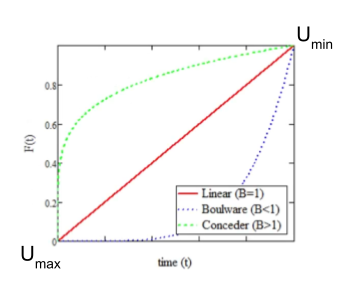
Formally, we define it like this:

Where F(t) is a function that takes in the time and returns a value between 0 and 1.
It gives the fraction of the distance between the best and the worst offer.
So for example, if F(t) = 0, we get Utarget(t) = Umax.
If F(t) = 1, we get Umin.
This function is defined as follows:

Tmax is the deadline, and β is a constant.
F(0) = 0, and F(Tmax) = 1.

Cool, but what’s β?
β determines what rate we’ll head towards the minimum at.

β → 0 - Hard-headed

No concessions; stick to the initial offer throughout (hope the opponent will concede)

β = 1 - Linear time-dependent concession

Linearly approach minimum utility

β < 1 - Boulware

Initial offer is maintained until just before deadline

β > 1 - Conceder

Concedes to minimum utility very quickly

Tit-for-tat

The agent detects the concession the opponent makes during the previous negotiation round, in terms of increase in its own utility function.
The drop in utility value of the offer the agent will concede to in the next round is equal to (or less than) the concession made by the opponent in the previous round:

If that made no sense, let me show you an example.
Your utility function is U(o) where o is an offer.
You make an offer to your opponent, o1, where U(o1) = 0.8.
Let’s say your opponent makes a counter-offer o2, and U(o2) = 0.5.
The next round, your opponent offers you a slightly better offer, o3, and U(o3) = 0.6.
So we like o3 slightly more than o2; by 0.1, to be exact.
That means, for our next offer, we can reduce the utility value for our initial offer by any value that is equal to or less than 0.1.
For example, our next offer could be o4 where U(o4) = U(o1) - 0.1 = 0.7.
Or it could be less: U(o4) = U(o1) - 0.05 = 0.75.

Basically, the rate at which our offers go down in our utility is the same / similar rate to which the opponent’s offers go up in our utility.

Uncertainty about the opponent

Imagine if you knew everything.
What would you do with that information?
One of the things you could do is give optimal concessions at any point in a negotiation.

If you really did know everything,

you probably wouldn’t be reading these notes.

But the reality is that we don’t know everything.
We don’t know exactly what our opponent likes and what they’re going to do.
However, we can create models of our opponent and guess what they’re like based on what they’ve done so far.

So now we have a target utility from the concession strategies, and we have a model of the opponent.
From those two, how do we create the best offers that’ll maximise our chance of getting an agreement we like?
We use an offer-producing strategy!

First, we create a graph of the agreement space:

Keep in mind that our opponent in this graph, agent 1, is just a model. An estimation.
Now let’s say our target utility is 8:

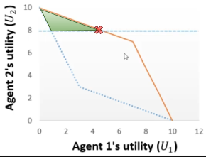
We want any offer in that shaded green region, because their utility values are all above / equal to 8.
However, it would be best to make the offer where the red X is.
That’s because it’s the offer that:

Satisfies our target utility
Is Pareto efficient
Maximises the opponent’s utility too, so they’re more likely to agree with it

When the opponent utility is not known, this is called private information.
We can guess the opponent’s utility function by looking at their behaviour.
For example, opponents are likely to concede on their least preferred issues first, so you can guess the weight of that issue.

Preference uncertainty

Sometimes we might not even know our own utility function.
“Huh? But I’m me! Of course I know my own utility function!”
But have a think about where the utility function actually comes from.

The utility function is just a mathematical model of your best interests, used by an agent.
The agent has to ask you a bunch of questions to optimise its utility function, but it’ll never perfectly map out your interests exactly.
This process is called preference elicitation.
Asking you questions is called cognitive costs.

If there’s a lot of possible outcomes, there’s a lot of questions the agent has to ask.
The agent wants to ask you lots of questions to get the best utility function that represents you, but it doesn’t want to bombard you with so many questions that it’ll take you the rest of your life just to answer them all.
So there’s a trade-off between cognitive costs and maximising the utility.

There’s also some recent work that looks at negotiation with incomplete information about our own utility, called preference uncertainty.
We’ll go into more detail about preference uncertainty later.

Utility Theory

A game is a mathematical model of interactive decision making.
Basically, agents go head-to-head and interact to try and achieve the best possible outcome.
There are different kinds of best outcomes, like winning, maximising payoff, etc.

An example of a game. Although the kind of

games we’re reasoning with are a bit simpler.

The kind of game we’ll be talking about will go like this:

An agent picks from one of a few finite decisions called choices.
When a choice is made, an outcome is reached (a.k.a result of their decision).
The outcomes could be anything:

Possible outcomes in a game of chess
Possible outcomes of negotiations between nations
Possible outcomes of an eBay auction

Let’s formalise some of this...

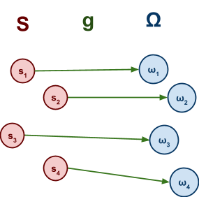
Let denote the choices available to an agent.
Let denote the outcomes.
Let denote the outcome function, which maps each choice to an outcome.

Alright, so in our formalised maths world, we can pick a choice and get an outcome.
But how do we know which choice will give us the best outcome?
To start off, we can model a preference between two outcomes.
In other words, given a pair of outcomes , we can say which one we prefer.

There’s actually two ways we can model preference:

Under certainty:

We know exactly what the consequences of our choices will be
For every choice, there is exactly one known certain consequence

Under uncertainty:

We don’t know exactly what the consequences will be
For every choice, there are multiple possible consequences, each with an attached probability

For now, we’ll focus on under certainty, because it’s the easier one.

Decision under certainty

A preference is a binary relation on .
So we can say if our agent prefers at least as much as .
We assume that it’s:

Reflexive

We prefer an outcome as much as itself.
for all

Total

We have to either prefer one outcome or the other.
For all , either or
(either or has to be true)

Transitive

If we prefer the second outcome over the first one, and the third outcome over the second one, then we’ll definitely prefer the third outcome over the first one.
For all , if and, then

When it satisfies all these properties, mathematics calls that a total preorder.

If and , then we are indifferent between the two.
That means we don’t care which one we pick.
We denote that with .

If but not , then we strictly prefer over .
That means we definitely prefer over .
We denote that with .

This outcome function is an ordinal preference.
We can also define something with cardinal preference.
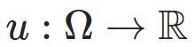
We can define a utility function, which maps an outcome to a numerical utility value.

A utility function over is said to represent a preference relation iff, for all :

iff

What does that mean?
With a preference relation, you can check if you prefer one outcome over another.
You can also do that with a utility function, by checking if the output of an outcome is greater than another.
So if you have a utility function that prefers all the same outcomes as a preference relation, you can say that utility function “represents” that preference relation.

Given a finite set , for every preference relation on there exists a utility function that represents it (basically, there’s always a utility function for every preference relation).

Keep in mind that agents do not choose outcomes based on the numerical value of the utility function; they choose it via their preference.
It doesn’t matter what the value is; the range could be between 1 to 10, or 1 to a billion.
We’re only using numerical values for adopting techniques for mathematical models, but keep in mind that only the relative order of the values is important.
Because the ranges of utility values aren’t defined, utilities of different agents cannot be compared.

Also remember that utility values are NOT money!
The difference is that with money, the value matters.
You’d say that going from £1 to £1,000 is way better than going from £1 to £10, right?
But if they were utility values, they’d both be equally as enticing, because it only matters that one number is bigger than the other.

Utility values are not legal tender and cannot be used in shops.

We can formally represent decision-making as a tuple:

Where:

and are the set of choices and consequences
is an outcome function that specifies the consequences of each choice
is the agent’s preference relation
is the utility function representing

A rational decision maker is one that makes the best possible choice.
That means the agent makes the choice that maximises their utility:

where

Don’t worry so much about the syntax; it just means we’re picking the choice that best maximises our utility function.
Because we’re using numerical utilities, we can express this decision problem as an optimisation problem.

Decision under uncertainty

When there is uncertainty, we don’t know what outcome will come from a choice.
When we make a choice, there are many possible outcomes, each with a probability of occurring.
Therefore a simple preference relation over two outcomes is not enough.
We need more!

To represent the uncertainty of an outcome, we use a probability distribution.
A probability distribution over a non-empty set of outcomes is a function:

such that:

So what does this mean?
It means that every outcome has a probability between 0 to 1.
If you add up all the probabilities of each outcome, it’ll sum up to 1 (naturally).
This whole concept is called a lottery.

Lotteries are denoted by .
For example, let’s say you sent a kid over to buy ice cream.
You tell the kid they can pick whatever flavour they like.
The probability distribution over what flavour they pick might look like:

As a lottery, this can be written as:

Mmmm, ice cream 🍨

When you think about it, a lottery is a generalised outcome.
If is the outcome of a choice , this is the same as a lottery where and, for all such that , (basically has a chance of 1 and all other outcomes have a chance of 0).
That lottery would be or just .
A lottery like that is called a degenerate lottery.

In the same way we can define a preference relation over a set of outcomes ...
... we can define a preference relation over a set of lotteries .
So say we could pick from between lottery L1 or lottery L2.
If we preferred L1 over L2, we could arbitrarily define .
We can also do the same with a utility function.

A compound lottery is a lottery of lotteries.
Given a set of lotteries , a compound lottery is a probability distribution over and is given by:

Where .

You want another example involving ice cream? Alright!

Let’s say you send the kid to get some ice cream again.
The kid has no money. You’re 70% sure it’s £1 a scoop, but you’re not totally sure.
You give the kid £1 anyway and send them to the ice cream van.
If a scoop is £1, the ice cream lottery takes effect:
If the scoop is more than £1, the kid can’t get anything, so this degenerate lottery takes effect:
As a whole, this is all one big compound lottery:

There’s another example about weather in the slides, but I wanted to expand on the previous example, and I also like ice cream.

The expected utility (EU) of a lottery is the average utility we can expect from that lottery.
It can be calculated like this:

Where:

is the set of outcomes
is the utility function
is the lottery
is the probability distribution of the lottery

What’s that? You want another example involving ice cream? Sure!

Let’s define a utility for each ice cream flavour:

Yeah yeah, you can argue about it in the Google docs comments.
Just a reminder, the probability distribution of the flavours go like this:

So we can calculate the EU of lottery L like so:
++
To simplify this, EU(L) = 2.1.

That’s great, but who cares?
Now, I know what you’re thinking.
“What’s the relation between preferences over lotteries and expected utility?”
What? You weren’t thinking that?
Well, von Neumann and Morgenstern were definitely thinking that.

A preference relation over outcomes is ordinal, and utility functions are cardinal.
A preference relation over lotteries is ordinal, and expected utilities are cardinal.
So you could try to think of things like this:

	Outcomes	Lotteries
Ordinal	Preference relation over outcomes	Preference relation over lotteries
Cardinal	Utility functions	Expected utilities

Utility functions can “represent” a preference relation over outcomes.
So can an expected utility “represent” a preference relation over lotteries?
Not exactly... there’s slightly more to it.

A preference relation over lotteries is arbitrary and vague.
We can just say if we prefer L1 to L2 and call it a day.
However, expected utilities (EUs) are calculated. It’s an actual value we can derive (as opposed to utility functions, where the value doesn’t matter).
Therefore these two aren’t really the same things in the same way that utility functions can “represent” a preference relation over outcomes.

Now don’t worry, von Neumann and Morgensten already found a relation between preference relations and expected utilities.
But we must define two axioms that preferences can satisfy first:

Continuity:

For every lotteries

there exist

such that

Independence:

For all lotteries

there exist

such that

Don’t worry so much if these don’t make sense. It’s only important that you know they exist.

The von Neumann - Morgenstern theorem goes like this:

Let be the set of compound lotteries over a finite set and let be a preference relation over . Then, the following are equivalent:

satisfies continuity and independence.
There exists a utility function over such that for all :

English please?
You can look at this in two ways:

If satisfies continuity and independence, then that means when
If when , then satisfies continuity and independence

If that still doesn’t make sense, don’t worry; just know that there is a connection between preference relations over lotteries and expected utilities.

Pure Strategy Games

Now, we’re going to be talking about strategic-form non-cooperative games.
Strategic-form non-cooperative games are games where:

Each player has different choices called strategies.
Players act alone, do not make joint decisions, and pursue their own goals.

Players simultaneously choose a strategy, and these combined strategies result in one of many outcomes.
Each player has their own preference over these outcomes.

Let’s give an example: The AB Game!

You are drugged one day, and you wake up in a warehouse.
You are wearing an electronic bracelet with the number “3” displayed on it.
If you can get the number to 9 or above, it comes off and you can escape.
If the number gets to 0 or below, you are killed.
To change the number on your bracelet, you need to play the AB game with others in the same situation as you.

When you play the AB game with someone, you both make two choices each, independently:

Ally
Betray

If you both pick “ally”, you both get 2 points.
If you pick “betray” and the other picks “ally”, you get 3 points and the other loses 2 points (and vice versa).
If you both pick “betray”, nobody gets any points.

Here, there are four possible outcomes for each player:

We can define a preference relation for each player such that:

It’s all like plus and minus and arghhh it’s confusing 🥴
It’d be easier if we assigned utility values to each outcome, so we can look and go “bigger number means better”

Strategic-form Games

Before we go on further, let’s formally define strategic form games a bit more.
A strategic-form game is a tuple:

Where:

is a finite set of players
is a finite set of strategies for each player
is a utility function for player ( is the set of reals)

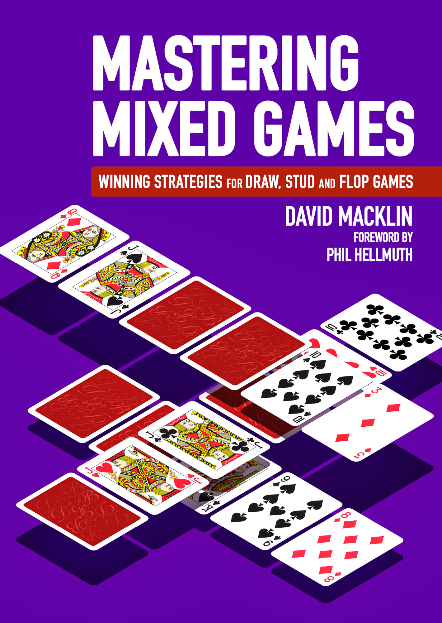
A strategy profile or strategy combination is a tuple:

It’s basically one of the possible combinations that players can pick their strategies.

They can also be denoted by:

... to highlight the strategy of player .
denotes the strategy combination without player :

is the set of all strategy combinations of the form excluding the player .
This syntax seems weird, but it’s just so we can focus on player .

Throughout this section, we assume that all players know each other’s strategies and utilities.
We also assume we’re all rational decision-makers.
A rational decision-maker is one that always chooses the option that maximises their utility.
With this in mind, how do we predict the outcome of these games?
We can define solution concepts, i.e. criteria that will allow us to predict solutions of a game under the assumptions we make about the players’ behaviour.

Strictly dominated strategies

So what sort of options will a player choose?
What if one of the choices always yielded worse results, no matter what happened?
You’d never pick that choice, right?
Therefore, we can rule out that choice.
That’s the main concept of strictly dominated strategies.

A strategy of player is strictly dominated if there exists another strategy of player such that for each strategy vector of the other players,

In this case, we can say that is strictly dominated by .
What this basically says is that if you pick strategy over , then no matter what the opponent picks, you’re gonna be missing out on some extra utility you could’ve gotten had you picked .
Because we’re assuming that players are rational, they’ll never pick strictly dominated strategies, so we can rule them out.

Let’s have a quick example:

Take a look at your “betray” strategy.
If you pick “betray” and they pick “ally”, you get an extra +2 utility that you wouldn’t have gotten had you picked “ally”.
If you pick “betray” and they pick “betray”, you get an extra +5 utility that you wouldn’t have gotten had you picked “ally”.
So no matter what, when you pick “betray”, you’re getting more utility than “ally”.
This means “ally” is strictly dominated by “betray”.
Therefore we can eliminate the “ally” strategy.
This is called iterated elimination of strictly dominated strategies.
We can eliminate these strategies in any order; it doesn’t matter.

So, according to this model, there’s really no reason to pick “ally”.
Although, I don’t think you’d have many friends if you followed models like these.

Weakly dominated strategies

Sometimes, there are no strictly dominated strategies.
What do we do then?
We can eliminate strategies where you either:

Miss out on utility had you picked another strategy
The utility you get is no different had you picked the other strategy

That’s the main concept of a weakly dominated strategy.

A strategy of player is weakly dominated if there exists another strategy of player such that:

For every strategy vector of the other players,

There exists a strategy vector of the other players such that,

In this case, we can say that is weakly dominated by .
What this basically says is that is at least as good as strategy .
When you pick over , depending on what the opponent picks, it will either not make any difference between picking or , or you’ll get more utility by picking over .
However, for it to be weakly dominated, there needs to be at least one strategy profile where picking over yields you more utility (so indifferent strategies can’t weakly dominate each other).

Let’s give another example:

Take a look at your “B” strategy.
If you pick “B” and they pick “C”, you’d get an extra +1 utility by picking “B” instead of “A”.
If you pick “B” and they pick “D”, it would’ve made no difference had you picked “B” or “A”.
This makes “A” weakly dominated by “B”.

We can eliminate weakly dominated strategies, and that’s called iterated elimination of weakly dominated strategies.
But there’s two things to remember:

The order of elimination matters; you could end up with different results!
You may eliminate some Nash equilibria from the game (more on this later).

Pure Nash Equilibria

Sometimes, there are no strongly / weakly dominated strategies to eliminate.
We can use a different concept, though.
The concept of stability: Nash Equilibrium!
But first, we need to define the concept of a “best response”.

Like the name suggests, a best response is the optimal strategy a player can take that maximises their utility, when used in response to the other player’s strategy.
Formally, let be a strategy vector for all the players not including . Player ’s strategy is called a best response to if:
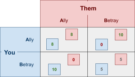
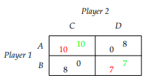
Take this example: let’s say you’re player 1, and player 2 just picked D.

What would be your best response?
If you look at the possible strategies:

Picking A would give you a utility of 0.
Picking B would give you a utility of 6.
Picking C would give you a utility of 3.

So picking B would be the best response to P2’s choice of D, because it’ll yield you the highest utility.

So now we know what a ‘best response’ is, what’s a Nash equilibrium?
A Nash equilibrium is a situation of stability in which both responses are best responses to each other.
Formally, a strategy combination is a Nash equilibrium if is a best response to for every player .
To illustrate this, I’m going to show the table again, but each green number is P2’s best response to P1, and each red number is P1’s best response to P2.

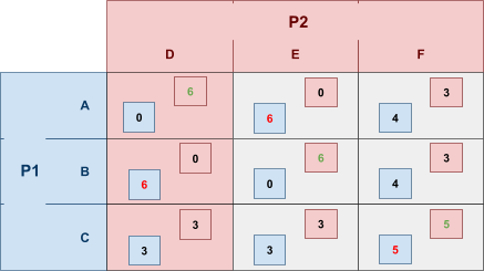
We can see that (C,F) are the best responses to each other!
Therefore, (C,F) is a Nash equilibrium.
This means if P1 picks C and P2 picks F, that means none of them will benefit from changing their choice, because they’ve already picked the best responses to each other.

How do we find these Nash equilibria?
There’s two main ways: best response intersection, and iterated elimination.
Let’s try the first for now: we find the best responses of both players, and we find the intersection.
Here’s the best responses for both players:

For player 1:
For player 2:

Now, we find the intersection of these two sets, and we have our Nash equilibria.
is shared between the two, so that’s our Nash equilibrium for this example.

It is possible that there might be multiple Nash equilibria.

A game with multiple Nash equilibria are called Coordination games.
Equilibria arise when players coordinate on the same strategy.
In addition, some games might not have any Nash equilibria, like the matching pennies game.

Now, we’ll go over that other strategy for finding Nash equilibria: iterated elimination.
If you perform iterated elimination of strictly dominated strategies and end up with one strategy profile to pick from, then that profile is a Nash equilibrium (and the only one in that game).

Eliminating strictly dominated strategies does not eliminate equilibria...
... but eliminating weakly dominated strategies might.

To put it more formally, given a game G, let G* be the game obtained by iterated elimination of weakly dominated strategies.
The set of equilibria of G* is a subset of the set of equilibria of G.
If you eliminate weakly dominated strategies, you may eliminate none, some, or all of the Nash equilibria in the game.
Here’s an example:

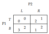
The equilibria are and .
In this example, we can eliminate L for being weak to R, and then eliminate B for being weak to T.
But... oops! We’ve eliminated the B row and L column. That means the Nash equilibrium is no longer present.

So remember, be careful with elimination. If you’re looking for Nash equilibria, it’s good to eliminate strictly dominated strategies, and then calculate the best responses for each player and then intersect.

Mixed Strategy Games

Before, in our pure strategic-form games, players could only pick one strategy and that’s it.
But what if we added a probability to each strategy?
What if you had, say, a 50% chance of picking one strategy and 50% chance of picking another one?
That is the core concept of mixed strategy games!

More formally, in a strategic-form game, a mixed strategy for player is a probability distribution over the set of strategies , i.e. a function such that

In other words, each strategy has a probability , which is the probability that player will play it. All strategy probabilities a player has must add up to 1 (naturally).
From now on, we’ll call these mixed strategies, and everything we had before we’ll call pure strategies.

Now, if you adopt a mixed strategy, you’ll be less predictable and keep your opponents guessing.
But when we had pure strategies, we could calculate Nash equilibria and stuff. How do we do that here? We’ll get on to that in a moment!

First, we need to introduce expected utility.
The expected utility of a mixed strategy is how much estimated utility you would get on average if you played that strategy.
It’s calculated using a weighted sum of pure utilities and probabilities.
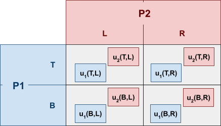
Here’s an example using Matching Pennies:

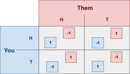
Let’s suppose that you play heads with probability of 0.4, meaning:

(because there’s only two options and 1 - 0.4 = 0.6)

... and our opponent plays heads with probability of 0.3:

What is our expected utility?
We need to do a weighted sum of every possibility that could happen in this game.
A weighted sum of probabilities and utilities.
Like this:

You pick heads and they pick heads
You pick heads and they pick tails
You pick tails and they pick heads
You pick tails and they pick tails

The expected utility for player 2 is calculated in a similar way.

Now to put all of this into maths syntax:
In a strategic-form game, for each player , let be the set of all mixed strategies over , i.e.

Let
We call every element a mixed strategy profile or mixed strategy combination.
In other words, contains every possible probabilistic strategy that each player could adopt in the game.
Like in pure strategies, we use to represent the strategies of everyone except player .
Given a mixed strategy profile , the expected utility of player is given by:

Let be a strategic-form game. The mixed extension of G is the game
Where:

Each is the set of mixed strategies of player over
Each (set of reals) is a payoff function that associates with each mixed strategy combination its expected utility (in other words, ).

Oof, that’s a lot of syntax...
That’s alright, though. As long as you understand the core concepts.

I wonder what the mixed Nash equilibrium of poker is?

(more on mixed Nash equilibrium later!)

Wait, what’s a mixed extension? We mentioned that above.
A mixed extension is a “new” game built on top of a strategic-form game with only pure strategies.
When you think about it, mixed games are actually just generalisations of pure games.
Pure games are just special forms of mixed games: in pure games, there’s one strategy for each player with probability of 1, and every other strategy is 0.
So if we have a pure game, we can actually treat it like a mixed game, with probabilities of 0 and 1. That’s what a ‘mixed extension’ means.

Mixed Nash Equilibria

To introduce the concept of Nash equilibria to mixed games, we need to define the concept of best response to mixed games first.

Let be a strategic-form game and let be its mixed extension. Let be a mixed strategy vector for all the players not including . Player ’s mixed strategy is called a best response to if

In other words, it’s a best response if there’s no other mixed strategy we can pick that’ll increase our expected utility.
It’s the same as the best response in pure games, except it’s about expected utility and mixed strategies, and not normal utility and pure strategies.

Now, defining a mixed Nash equilibrium is easy.
A mixed strategy combination is a mixed strategy Nash equilibrium if is a best response to for every player .
Like in pure games, a mixed strategy Nash equilibrium is where both responses are best responses to each other (but this time, it’s mixed).
We’ll use the term “mixed Nash equilibrium” to refer to this, and “pure Nash equilibrium” to refer to the Nash equilibrium defined in “Pure Strategy Games”.
Naturally, since pure games are special kinds of mixed games, pure Nash equilibria are special kinds of mixed Nash equilibria.

In our matching pennies game, there is a unique mixed Nash equilibrium, and that’s to pick heads 50% of the time, and tails the other times, for both players:

Hype for competitive Matching Pennies at the next Olympics

In pure games, pure Nash equilibria do not always exist. Sometimes there are none.
However, in a mixed game, there is always mixed strategy Nash equilibria.
It’s pretty hard to find them, though. It’s PPAD-complete (Daskalakis, Goldberg, Papadimitriou, 2009)!
It’s not so hard to find them in 2x2 games, though. That’s what we’ll focus on.

Computing Mixed Nash Equilibria

First, let’s define a generic 2x2 mixed game.

The probabilities of player 1 (P1) are:

Picking T:
Picking B:

The probabilities of player 2 (P2) are:

Picking L:
Picking R:

Both and are in the range , as a probability normally would.

Best Response Method

This is the first method of finding Nash equilibria.
What we do is we construct functions for each player’s best response:

The intersection between these functions will give us our mixed Nash equilibria.

Let’s walk through an example while I explain:

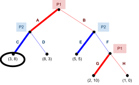
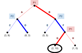
Here, we have 2 pure Nash equilibria and , but also a mixed Nash equilibrium that we want to find.
Let’s start with player 1.
Player 1’s best response is:

What does “argmax” mean?
It stands for “arguments of the maxima”, and it means its selecting a value of that maximises , and returning that instead.
So you can think of as the “best value of that maximises our expected utility”.

So how do we get the best values of ?
First, let’s simplify using our equation and go from there:

So, it seems that our best value of (the value of that maximises our expected utility) depends on the value of .
Have a closer look at our equation. is the coefficient of the only term.
If is negative, then as we increase , our expected utility will get smaller. So, we would need to pick the smallest we can, which is 0.
If is positive, then as we increase , our expected utility will get bigger. So, we would need to pick the biggest we can, which is 1.
If is zero, then no matter what value of we pick, our expected utility stays the same (because is getting cancelled out). Therefore we can pick any value of , even 0 and 1. In other words, the range [0,1] (between 0 and 1, and including them; ‘inclusive’).

So now our best values of looks like this:

You know, we can rearrange that coefficient to isolate :

That’s it! We’ve got the best values of .

Now we need to find the best values of .
This is more-or-less the same as finding the best values of , so I’ll skim it a bit.

Yatta! We’ve got the best values of and now.
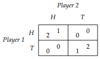
There’s one step now: plotting the best results and finding intersections.

As you can see, there are three intersections, representing the three Nash equilibria:

The pure Nash equilibrium for
The pure Nash equilibrium for
The mixed Nash equilibrium for , or

Indifference Principle

This method is a bit more numerical.
It’s based off the indifference principle, which goes like this:

Let be a mixed Nash equilibrium of a strategic-form game, and let and be two pure strategies of player . If

then

In other words, if you have a mixed Nash equilibrium and multiple pure strategies have probabilities greater than 0, then each of those pure strategies have the same payoff.
They are indifferent to playing a pure strategy over another.

We call a mixed strategy of player a completely mixed strategy (or fully mixed) if

... for every pure strategy .
In other words, a completely mixed strategy is where every pure strategy has some probability higher than 0.
We call a mixed Nash equilibrium a completely mixed Nash equilibrium (or fully mixed) if for every player , the strategy is completely mixed.
So if our mixed Nash equilibrium contains all fully mixed strategies, we call it a completely mixed Nash equilibrium: a special kind of mixed Nash equilibrium. Pretty simple, right?

Let’s refer back to our generalised 2x2 game again.

As usual, is the probability P1 will pick T, and is the probability P2 will pick L.
Let’s define some helper functions:

is the expected utility for P1 when choosing T,
is the expected utility for P1 when choosing B, and so on.

Now, here is how our indifference principle method works:

A pair of probability distributions is a completely mixed Nash equilibrium in the generic 2x2 game if and only if

This is just an application of the indifference principle on our generalised 2x2 game.
The expected utility for P1 when choosing T is the same as the expected utility for P1 when choosing B, and so on for P2.
There is a proof for this, but it’s not examinable.

We first check the first equality and find solutions for .
We then check the second equality and find solutions for .
Lastly, all pairs of solutions are fully mixed Nash equilibrium.
Because this is a game with only 2 strategies for each player, all fully mixed Nash equilibria are also just normal mixed Nash equilibria. If we had more strategies for each player, that wouldn’t be true.

One difference between best response method and indifference principle method: the best response method can find both pure and mixed Nash equilibria, but the indifference principle method can only find fully mixed Nash equilibria.

Let me guess: you want an example?
You got it!

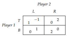
There are no pure Nash equilibria here.
First step:

Second step:

So is a fully mixed Nash equilibrium.

Let’s look at an example where this doesn’t work.

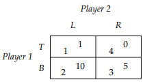
is a pure Nash equilibrium here.
First step:

Second step:

Uh oh... 5/4 is not a valid probability.
😳 awkward
That means there are no completely mixed Nash equilibria in this example.

One more example: this time, we will use indifference principle to verify if a strategy is a fully mixed Nash equilibrium.

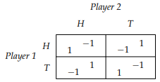
Let’s say we’re trying to verify if is an equilibrium.
We can try plugging them into our expected utility functions to see if the two values are equal.
If is supposed to be true for fully mixed Nash equilibria, let’s try subbing our value of into that and see if it all holds up.

Ah... that doesn’t look right.
Because they’re not equal, this strategy cannot be a mixed Nash equilibrium.

Extensive-Form Games

In strategic-form games (pure games and mixed games), players make a move simultaneously, e.g. both players pick “Ally”.
However, we’re going to look at extensive-form games, where players make moves sequentially in turns.
There are different models of decision-making:

Games with perfect information: players know exactly how the current state of the game was reached
Games with imperfect information: players may be uncertain about previous moves, may not know how the current state was reached
Games of perfect recall: no player forgets the action they previously chose

We will only focus on games with perfect information.

Again, an extensive-form game is a game where each player takes turns, and the previous actions determine the current possible actions.
Like how we represented strategic-form games with a table, we can represent extensive-form games as a tree:

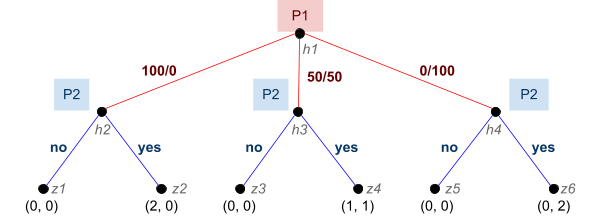
We’ll call this example the Ultimatum game.
It goes like this:

P1 suggests one of three possible splits of a cake:

P1 gets all, P2 gets none
P1 gets half, P2 gets half
P1 gets none, P2 gets all

P2 can either accept or reject the offer

The game starts at the root (the node at the very top), and goes through each arc, which represent the choices that each player takes, until we reach a leaf node, which represents an outcome.
Each node belongs to a player, at which that player has to make a decision when the game reaches that node.
The leaves are the outcomes, and result in utilities for the different players.

Let’s define things formally.
A finite extensive-form game with perfect information is a tuple

... where:

is a finite set of players
is a (single) set of actions
is a set of non-terminal choice nodes
is a set of terminal nodes, disjoint from H
is the action function, which assigns to each choice node a set of possible actions.
is the player function, which assigns to each non-terminal node a player who chooses an action at that node
is the successor function, which maps a choice node and an action to a new choice node or terminal node such that for all and , if , then and .
, where (set of reals) is a real-valued utility function for player on the terminal nodes .

In the ultimatum game, these values are:

Players:
Actions:
Choice nodes:
Terminal nodes:
Action function:

Player function:

Successor function:

Utility function:

Phew... that was a lot to type out.

Ever noticed how Computer Science tables and trees

look nothing like their real-life counterparts?

Just like how we can have strategies in strategic-form games, we can have strategies in extensive-form games.
A pure strategy in an extensive-form game contains the choices a player is going to make at any of their nodes in the game.
For example, in the ultimatum game, P1’s strategy can only cover the one node P1 makes a choice in: h1. So P1 can only adopt one of three strategies: 100/0, 50/50, or 0/100.
For P2, it’s a bit different. P2 has three nodes at which they can make a decision, so their strategy needs to account for those.
P2 can pick strategy (yes,yes,yes), or (no,no,yes), or any combination of three no’s and yes’, with the first, second, and third elements of the tuple representing the choices at h2, h3, and h4, respectively.

More formally, the pure strategies of player consist of the Cartesian product

Therefore, the strategy of P1 is:
The strategy of P2 is:

Strategic-Form Transformation

Now that we have pure strategies in extensive-form games, we can map strategy profiles to player utilities, depending on what outcome node those strategies will end up at.
By doing this, we can convert extensive-form into strategic-form.
Here’s an example:

Strategies for P1:

Strategies for P2:

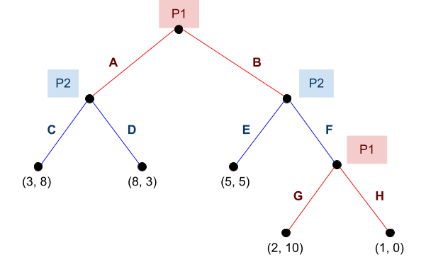
Now, we put these into a table, with each player’s strategies being their own axis:

	(C,E)	(C,F)	(D,E)	(D,F)
(A,G)	3 / 8	3 / 8	8 / 3	8 / 3
(A,H)	3 / 8	3 / 8	8 / 3	8 / 3
(B,G)	5 / 5	2 / 10	5 / 5	2 / 10
(B,H)	5 / 5	1 / 0	5 / 5	1 / 0

You can get these utilities by following the strategies through the tree, and finding the utility of the outcome node the strategies lead to:

	(C,E)
(A,G)	3 / 8

	(D,F)
(B,G)	2 / 10

It’s always possible to convert extensive-form to strategic-form.
However, this negates the temporal nature of the game.
In the original extensive-form version, we had 5 outcomes. In its converted strategic-form, we have 16.
By converting, we add a bunch of redundant outcomes.
Also, remember that it’s not always possible to convert strategic-form to extensive-form.

Equilibria

Now that we know extensive-form games can be converted to strategic-form games, we can compute pure Nash equilibria for extensive-form games.
Unlike strategic-form games, there is always pure Nash equilibria in extensive-form games.
More formally, given any finite perfect-information extensive-form game G, let G* be its strategic-form. Then G* has a pure strategy Nash equilibrium (Zermelo, 1913).

So, the plan is: convert extensive-form to strategic-form, then calculate pure Nash equilibrium. Easy, right?
Then let’s try it with our example from above.

	(C,E)	(C,F)	(D,E)	(D,F)
(A,G)	3 / 8	3 / 8	8 / 3	8 / 3
(A,H)	3 / 8	3 / 8	8 / 3	8 / 3
(B,G)	5 / 5	2 / 10	5 / 5	2 / 10
(B,H)	5 / 5	1 / 0	5 / 5	1 / 0

The pure Nash equilibrium are ((A,G),(C,F)), ((A,H),(C,F)), and ((B,H),(C,E)).
Wow, that was so easy!
... or was it?

Let’s have a look at ((B,H),(C,E)) in terms of the original extensive-form game.

Some of these choices are fine, like when P2 picks C over D because it maximises their utility.

However, look at P1 picking H over G. Why would they do that? They’re getting a utility of 1 instead of 2. They’re minimising their own utility.

I know that choice doesn’t affect things in this strategy, but is that the sort of behaviour you’d expect from a Nash equilibrium?

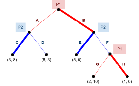
Hint: the answer is no.
Alright, so pure Nash equilibrium are a bit dodgy when you get them from an extensive-form game’s strategic-form game equivalent.
But it’s still pure Nash equilibrium. It just looks bad in a different context.
We need something better... something that incorporates the fact that it’s an extensive-form game.
We need...!

subgame perfect equilibria

You hear that? It’s literally got “perfect” in the name. How bad could it be?
But first, we need to introduce the concept of subgames.

It’s pretty simple, really. A subgame is like a subtree of an extensive-form game tree. It is a restriction at one of the non-terminal nodes.
More formally, given a perfect-information extensive-form game G, the subgame of G rooted at node h is the restriction of G to the descendants of h.
The set of subgames of G consists of all subgames rooted at some node in G.

To find all the subgames of an extensive-form game, just look at all the non-terminal nodes and make them into roots of their own subgames.
Here’s all 4 subgames of our example:

Yes, the game is its own subgame.

A subgame perfect equilibrium is a pure Nash equilibrium of an extensive-form game that is also a pure Nash equilibrium of all of its subgames.
More formally, a strategy profile in an extensive-form game is a subgame perfect equilibrium if, for each subgame of , the restriction of to is a pure strategy Nash equilibrium.
Every extensive-form game has a subgame perfect equilibrium.
The set of subgame perfect equilibria is a subset of the set of pure Nash equilibria.

So how do we find subgame perfect equilibria in our example?
We have three pure Nash equilibria, and every extensive-form game has a subgame perfect equilibrium, so at least one of those three equilibria must be subgame perfect.
Let’s go through each one and check if they’re subgame perfect!

((B,H),(C,E))

((A,H),(C,F))

No, these strategies are not subgame perfect.

Why? Because in the subgame with just G and H, P1 picks H and gets a utility of 1 instead of picking G and getting a utility of 2.

P1 can maximise their utility by picking a different pure strategy, so in this subgame, it’s not a Nash equilibrium.

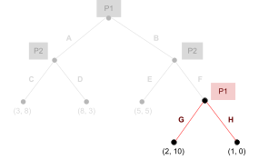
((A,G),(C,F))

Let’s go through each subgame and see if this strategy is a Nash equilibrium in all of them.

	N/A
G	2 / 10
H	1 / 0

G is a Nash equilibrium in this subgame.

In our strategy, P1 plays G in (A,G), so our strategy is a Nash equilibrium in this subgame.

	C	D
N/A	3 / 8	8 / 3

C is a Nash equilibrium in this subgame.

In our strategy, P2 plays C in (C,F), so our strategy is a Nash equilibrium in this subgame too.

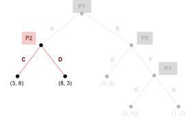
	E	F
G	5 / 5	2 / 10
H	5 / 5	1 / 0

(G,F) and (H,E) are Nash equilibrium in this subgame.

In our strategy, P1 plays G in (A,G) and P2 plays F in (C,F), so our strategy is a Nash equilibrium in this subgame.

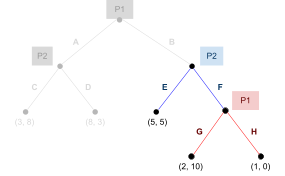
It seems like ((A,G),(C,F)) is a Nash equilibrium of the whole game and all its subgames, making it a subgame perfect equilibrium.

Backward Induction

Do you seriously want to find all the pure Nash equilibria, and then go through them all, checking each one if they’re subgame perfect?
That’s inefficient and long and boring and cringe.
There’s an algorithm for finding subgame perfect equilibria; one that doesn’t involve converting to strategic-form.
Introducing Backward Induction!

It’s like mathematical induction, but instead of dominos, it’s, uh... trees.

Backward Induction is an algorithm for finding subgame perfect equilibria that involves computing each small subgame and replacing them with the reasonable utility, all while storing the best choices and compiling a subgame perfect strategy, until we reach the root and finish.
Here are the steps in more detail:

Take the tree representing an extensive-form game with players.
Starting from the smallest subgames (i.e. those rooted at nodes whose children are terminal nodes), compute the Nash equilibrium for the player making the choice
Replace the subgame with utility obtained, i.e. make the node of the subgame a terminal node and label it with the utility of the equilibrium.
Repeat the process for every subgame rooted in a node leading to terminal nodes, i.e.: compute the Nash equilibrium and replace the game with the result of its equilibrium.
If at any step a subgame has multiple Nash equilibria (i.e. when the utilities of different choices are the same), select any of them.
The algorithm terminates when we reach the root node of the whole game and runs in polynomial time in the size of the tree.
For every player , let be the vector where each component is the choice made by the player in the process of selecting the equilibrium of a subgame.
is a subgame perfect equilibrium and the utility at the root node is the value of the equilibrium.

What? Reading is boring?
You want to see the pictures with the pretty colours?
Then let’s apply Backward Induction with our example from above:

((_,G),(_,_))

First, let’s look at this subgame on the right. P1 is playing, and naturally, they’d want to maximise their utility.

That means P1 would want to pick the left choice ‘G’, right? They’d get a utility of 2 instead of 1.

Therefore, P1’s choice at this node is G, and we replace this non-terminal subgame root node with a terminal node of utility (2,10).

((_,G),(_,F))

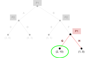
Now, let’s look at the next subgame on the right. P2 is playing, so they’d want to maximise their utility.

P2 would pick the right option ‘F’, so they’d get a utility of 10 instead of 5.

So, like before, we remember that P2 should pick F at this node, and replace this subgame with a terminal node of utility (2,10).

((_,G),(C,F))

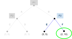
Let’s look at the subgame on the left. Again, P2 is playing.

P2 should pick ‘C’, as they’ll get a utility of 8 instead of 3. This subgame will be replaced with (3,8).

((A,G),(C,F))

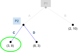
This is the final subgame! P1 is playing.

P1 should pick ‘A’, as they’ll get 3 instead of 2.

Since this is the final subgame, we have now compiled our entire strategy. This strategy is subgame perfect, and will yield P1 and P2 utilities of 3 and 8, respectively.

Do you wanna do this with the ultimatum game?
There’s a step-by-step in the slides, but I’ll just spoil you here.
There are two subgame perfect equilibria:

(50/50, (no,yes,yes))
(100/0, (yes,yes,yes))

In the general version of the ultimatum game, where P1 can split the cake into n slices, there are still two subgame perfect equilibria:

One where P1 takes it all, leaving P2 with none, and P2 says yes at every node
Another where P1 takes n - 1 slices, leaving P2 with 1 unit of cake, and P2 says yes at every node, except the one where P1 takes everything

Yikes... things are really unfair for P2.

There’s also this weird centipede game:

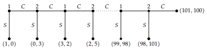
... where if P1 stops the game, the payoff is (t, t - 1), and if P2 stops the game, the payoff is (t - 2, t + 1), and the game abruptly ends if nobody stops before 100 rounds pass.
The only subgame perfect equilibrium here is the strategy where P1 and P2 try to stop the game at every stage.
But that means the payoff will be a measly (1,0). They could get way more if they play for a bit longer!
Sometimes, even the subgame perfect equilibrium is unreasonable. Remember, these are all just mathematical models created to reason with problems we make up. In the real world, there’s way too many variables to consider.

I wanted to put a picture of a centipede here, but I couldn’t find a good or cute picture of a centipede; only disgusting ones, so here’s a clipart caterpillar instead.

Linear Programming

A lot of the linear programming section was already covered in Algorithmics.
Be sure to check out that section if you never did Algorithmics, or need a refresher.

Some famous methods of solving LP problems are:

Simplex method

Worst-case time complexity: exponential
Average time complexity: O(n3)

Ellipsoid method

Polynomial-time
Generally slow, so cannot compete with Simplex

Karmarkar’s algorithm

Polynomial-time
Runs fast with large inputs, sometimes faster than Simplex

If we’ve done this before, why are we learning this again?
Does Bahar want to get a kick out of teaching us stuff we already know?
Not quite; there’s a way to apply linear programming to Nash equilibrium.
We can use it to compute a Nash equilibrium of a two-player zero-sum game.
How do we do that? I’ll show you...

Computing Nash Equilibrium with LP

Remember that the game must be:

Two-player: there are only two participants in the game
Zero-sum: one’s gain is another’s loss

Let’s give an example:

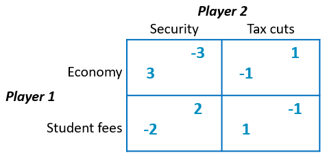
Firstly, we will calculate player 1’s strategy.

A mixed strategy of player 1 is represented as (x is probability of picking “economy”, so 0 means “definitely student fees” and 1 means “definitely economy”)
The expected payoff of player 1 will be:

if player 2 picks “security”
if player 2 picks “travel cuts”

What will player 2 do?
Here, we’ll assume that player 2 picks a pure strategy.
That means either definitely “security” or “tax cuts”.
Which one will player 2 pick?
Player 2 will pick the one that maximises their utility.
Because it’s a zero-sum game, when player 2 maximises their utility, that also means they’re minimising player 1’s utility (because player 1’s loss is player 2’s gain).
So player 2 will pick one that minimises player 1’s utility.

This means player 1’s expected utility will be :

Player 1 should pick a value of ‘x’ that maximises this.

Now we can convert this into an LP problem!
Let’s call player 1’s minimum expected utility ‘z’:

Let’s convert it to an LP problem:

maximise: z
subject to:

If you’re wondering about the first two constraints, we’re minimising ‘z’ with the expected payoffs to model the “min” part of our expected utility. Basically, the min function will pick either or , making (min’s choice - z) = 0. The other one will be larger, so (the other one - z) will be greater than 0.
The solution to this is:

z = 1/7
x = 3/7

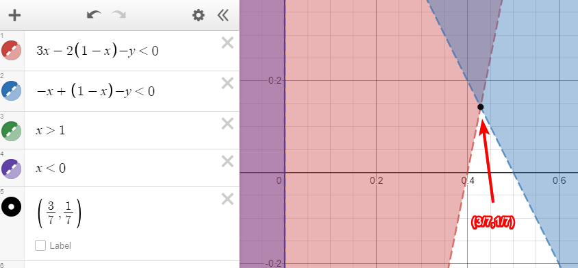
So player 1 should play economy with probability 3/7 and student fees with probability 4/7.
In other words, the calculated strategy is (3/7, 4/7).

Now that we’ve calculated player 1’s strategy, we can calculate player 2’s.
We do it in pretty much the same way.
Player 2’s mixed strategy is (where y=0 means “definitely tax cuts” and y=1 means “definitely security”).
The payoff of player 2 will be:

if player 1 picks “economy”
if player 1 picks “student fees”

Let’s say player 1 picks a pure strategy. They’d pick one to minimise player 2’s utility.
So player 2’s minimum expected utility is:

Now let’s convert this to an LP problem:

maximise: w
subject to:

The solution to this is:

w = -1/7
y = 2/7

So player 2 should play security with probability 2/7 and tax cuts with probability 5/7.
In other words, the calculated strategy is (2/7, 5/7).

Have a look at the two minimum expected utilities we just calculated.

Player 1’s z = 1/7
Player 2’s w = -1/7

The sum of these two is 0, showing that this game is zero-sum (naturally).

Since the game is zero-sum, what one gets (x), the other loses (-x).
If player 2 plays our calculated strategy of (2/7, 5/7), that means player 2 can get a minimum utility of -1/7 (the value of w we got). Because player 2 gets minimum -1/7, player 1 gets maximum 1/7.
Likewise, If player 1 plays (3/7, 4/7), that means player 1 can get a minimum utility of 1/7, which means player 2 gets a maximum utility of -1/7.
None of the probabilities are zero, which means (3/7, 2/7) is a fully mixed Nash Equilibrium.

Structure of linear programs

The constraints in a linear program describe a convex polytope in n-dimensional space.
The convex polytope is the shape, or the perimeter, of the linear program when you plot it into a graph.
It corresponds to the feasible region that consists of all feasible solutions (the edges and the inside of the convex polytope contains all solutions).
The objective function will attain its minimum / maximum at a vertex of the polytope (the best solution / optimum is always on the edge, never on the inside).

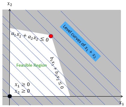
Unique solutions

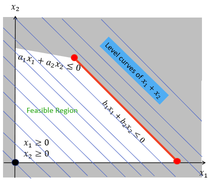
Multiple solutions

The set of constraints may be infeasible, which means there are no solutions.
A linear program is unbounded if there are feasible solutions, but there’s no finite optimal objective value (a.k.a it goes on infinitely; there’s always a better value no matter what you pick).

Unbounded solutions

Transforming linear programs

There are two forms of linear programs:

Standard form

Maximisation using inequalities (≥, ≤)
They have the following format:

So they:

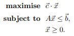
Must maximise
All linear constraints must have ≤
All non-negativity constraints must have ≥.

e.g:

maximise x
subject to

3x + 2y + z ≤ 5
4x + 7y + 7z ≤ 20
x ≥ 0
y ≥ 0
z ≥ 0

Remember that strict inequalities are not allowed in linear programs!
That means no > or <.

Slack (normal) form

Maximisation using equalities (=)
e.g:

maximise x
subject to

3x + 2y + z - s1 = 5
4x + 7y + 7z + s2 = 20
x ≥ 0
y ≥ 0
z ≥ 0

You can introduce slack variables,

but you can’t procrastinate from work with them.

We can convert standard form to slack form by introducing slack variables:

a + b + c ... < x → a + b + c ... + s1 = x (+ s1 = deficit)
a + b + c ... > x → a + b + c ... - s2 = x (- s2 = excess)

We can convert an equality constraint into two inequality constraints:

a + b + c ... = x →

a + b + c ... ≥ x
a + b + c ... ≤ x

But remember that in standard form, linear constraints must have ≤, so be sure to flip the sign:

a + b + c ... ≥ x →

- a - b - c ... ≤ -x

If you have a non-negativity constraint that’s the wrong way (≤ instead of ≥), flip the sign, and minus the variable across the LP:

maximise x
x + y + z ≤ 7
x ≤ 0 →

maximise -x
-x + y + z ≤ 7
x ≥ 0

If there are no non-negativity constraints on a variable (basically, it can be any value), we can replace it with two non-negative variables:

x (x can be anything) → x’2 - x’’2
x’2 ≥ 0
x’’2 ≥ 0

Beyond linear programming

There’s variations to linear programming:

Integer linear programming: the same as LP, but all variables must be integers.

NP-hard to find a feasible solution

Quadratic programming: linear constraints, but a quadratic objective function.

Can be solved in polynomial time
Ideas are similar to LP
Important applications in science and engineering

Preference Elicitation

Here, we’ll be going into detail about preferences. If you need a refresher, take a quick read here.

Here are some transitivity rules:

If x ≽ y and y ≽ z then x ≽ z
If x ∼ y and y ∼ z then x ∼ z
If x ≻ y and y ≻ z then x ≻ z
If x ≽ y and y ≻ z then x ≻ z
If x ≻ y and y ≽ z then x ≻ z

Preference ordering

We can chain these relations to make a preference ordering.
Here’s what an ordering looks like:

x ≻ y ≻ z ~ a ~ b ≻ d ≻ c ~ e

They’re alternated in red and blue to make it easier to see what elements are in what order.
Do you see some orderings where there are consecutive elements of the same “colour block” (like z,a,b or c,e)?
That’s called a tie (or equivalence class). It means they’re all equivalent in terms of ordering.
For example, y is preferred to either z, a or b. Also, any of z, a or b is preferred to d.

Transitivity is nice, because it makes logical sense.
If you like strawberry over vanilla, and vanilla over chocolate, you’re obviously going to prefer strawberry over chocolate.
However, when we aggregate preferences, we might run into problems.

Let’s have another example involving ice-cream:

Phoenix: strawberry ≻ vanilla ≻ chocolate
Miles: vanilla ≻ chocolate ≻ strawberry
Larry: chocolate ≻ strawberry ≻ vanilla

Let’s say these three fully-grown, mature adults only have enough money for one ice-cream to share.
So they decide to aggregate their preferences and make a decision.
However, there are some contradictions...

Phoenix likes strawberry over vanilla, whereas Miles prefers vanilla
Miles likes vanilla over chocolate, whereas Larry prefers chocolate
Larry likes chocolate over strawberry, whereas Phoenix prefers strawberry

So we can’t just throw these preferences together and hope they work together, because transitivity would break down.
There’s ways of aggregating preferences properly, but we’ll go over that later.
For now, we assume transitivity!

Preference uncertainty

Like we said before, we don’t know everything.
We don’t always know our own preference.
It can be costly to find out as well; we’d be spending our budget of:

Time
Money
Cognitive cost

If it’s too costly to fully rank our entire preference, we can invest our budget on partially learning it.
Our budget put towards partially learning our preference is called the elicitation budget.

We usually start off with some partial information (or none at all).
Then, we make a bunch of queries to build our preference profile.
There’s two kinds of queries we can ask:

Pairwise queries: compare two given outcomes

e.g:

Do you prefer strawberry or vanilla?
Do you prefer chocolate or mint choc chip?

Given n outcomes...
Worst case, you need n log n pairwise queries to map out your full ordering (because comparing two options is basically just sorting).
Best case, you need n - 1 pairwise queries to map out your full ordering (if every option you compare is always better / worse than the last).

Interviews: learn as much as possible about the value of an outcome

e.g:

On a scale of 1 to 10, how much do you like rum and raisin?
On a scale of 1 to 10, how much do you like bubblegum?

Given n outcomes, worst case and best case, you need n interviews to map out a full ordering.

As great as interviews sound, they are way more expensive than pairwise queries.
A lot less computation needs to go into picking one or the other.
A choice (pairwise query or interview) will depend on the application, and sometimes a combination of both will be used.

Use pairwise queries if two outcomes are sufficiently distinct
Use interviews if outcomes are similar and need more info to rank them

An elicitation scheme / strategy / plan describes what queries to ask and when.
The plan may:

depend on the previous question / query
depend on the state of the universe / game

We’ve always assumed that the result of a query is deterministic.
If I ask you “do you prefer vanilla or mint choc chip?” and you say “vanilla”, I might assume you will always prefer vanilla.
However, what if you’re suddenly in the mood for mint?
Or you get cravings?
Or you suddenly become allergic to vanilla?
Then, you’ll answer “mint choc chip” to my question.

I wanted to reference some other flavours,

but there weren’t enough unique text colours.

The point is, queries can be probabilistic.
The pairwise queries of vanilla and mint choc chip might end up like:

p(vanilla ≻ mint choc chip) = 0.7
p(mint choc chip ≻ vanilla) = 0.3

The interviews of strawberry, vanilla and chocolate might end up like:

p(strawberry ≻ vanilla ≻ chocolate) = 0.2
p(vanilla ≻ chocolate ≻ strawberry) = 0.5
p(chocolate ≻ vanilla ≻ strawberry) = 0.3

However, in the following sections, we’ll always assume they’re deterministic.
We’ll also only use pairwise queries.

Multi Criteria Ranking using Multi-Attribute Additive Functions

In Multi-Criteria Decision Analysis (MCDA), we evaluate outcomes based on a set of criteria or “issues”, where:

(set of reals)

... is the evaluation of issue in outcome , for all and .
The greater is, the better outcome is on issue .
We can rank our outcomes based on these issue evaluations.
In other words, each outcome has a bunch of “issues” that we can evaluate and compare with.

To give an ice-cream related example:

Flavours	Sweetness g1	Texture g2	Richness g3
Strawberry	70	60	20
Vanilla	60	60	30
Chocolate	40	50	80

So, for example, g3(vanilla) = 30.

The utility of an outcome can be represented as an additive value function, such as:

... where is a non-decreasing marginal value function for issue (this may seem useless, but we’ll see exactly why we use this later).
Let’s see an example, given that is the identity function (it never is, but let’s pretend):

U(strawberry) = u1(g1(strawberry)) + u2(g2(strawberry)) + u3(g3(strawberry))
U(strawberry) = u1(70) + u2(60) + u3(20)
U(strawberry) = 150

I’m going to use ui(o) instead of ui(gi(o)) from now on, for simplicity.
Value functions are increasing with respect to preference ordering, e.g:

strawberry ≻ chocolate ⇔ U(strawberry) > U(chocolate)
strawberry ∼ chocolate ⇔ U(strawberry) = U(chocolate)

We can even add weights to these functions.
For example, if you prefer the sweetness of a flavour over its texture, you could grant sweetness a heavier weight than texture.

This is just one of the many ways you could design the functions.

This is all looking very familiar...

Ordinal Regression via Linear Programming (UTA)

Ordinal Regression is the process of finding a possible value function U that satisfies some partial information that is already known, and using that function to generate a complete preference ordering.
With ordinal regression, we initially have no function for ui, but we already have a function for gi.

For example, say we have a bunch of flavours: strawberry, vanilla, chocolate, mint choc chip, rum and raisin, bubblegum.
We already know that mint choc chip ≻ bubblegum ≻ vanilla, and we have gi, but not ui.
Therefore, we gotta try and locate a possible U that satisfies (or is compatible with) mint choc chip ≻ bubblegum ≻ vanilla.
In other words, a U such that U(mint choc chip) > U(bubblegum) and U(bubblegum) > U(vanilla).
We then use that U to map out our entire preference ordering.

There are two methods that do this:

UTA: additive ordinal regression

Assumes agent knows a complete preference ordering over a set of reference outcomes / alternatives .
Among the possible additive value functions that are compatible with the partial preference information, one is picked and used to generate a complete preference ordering over all outcomes.
Assumes that all ui’s are piecewise-linear (more on that later).

UTAGMS: robust additive ordinal regression

The ranking of reference outcomes does not need to be complete.
Takes into consideration all compatible additive value functions.
ui’s are general non-decreasing functions.

If a lot of that just went over your head, don’t worry; we’ll go into way more detail.

Contrary to popular belief, the UTA method was not invented in Utah.

Let’s start off with normal UTA.

First of all, the agent has a complete preference ordering over a set of reference outcomes .
Basically, the agent knows a complete preference profile over a small group of outcomes.
A good example is:

mint choc chip ≻ bubblegum ≻ vanilla

Where

OR = {mint choc chip, bubblegum, vanilla}
O = {strawberry, vanilla, chocolate, mint choc chip, rum and raisin, bubblegum}

More formally, for every two outcomes c and d in OR, one of these must be true:

c ≽ d “c is at least as good as d”
c ≻ d “c is preferred to d”
c ∼ d “c is indifferent to d”

A value function U is compatible iff, for each c and d in OR:

U(c) ≥ U(d) ⇔ c ≽ d
U(c) > U(d) ⇔ c ≻ d
U(c) = U(d) ⇔ c ∼ d
Basically, compatible means that the value function U yields the same ordering as the preference relation ≻.

The range of gi is [αi, βi], where αi < βi.

This is basically saying that for each issue i, the function gi has a finite range, and the lower and upper limits of that range is αi and βi respectively.
αi is the worst finite evaluation for the issue.
βi is the best finite evaluation for the issue.

This range is divided into γi > 1 equal subintervals.

Each subinterval edge is represented as , where j = 1...γi.
For example, let’s say i = 1 (sweetness), αi = 0, βi = 100 (making the range [0,100]), and γi = 4.
That means there’d be 4 subintervals, each of size 25.
The subinterval edges would be:

The marginal value of an outcome on an issue is obtained via linear interpolation.

When getting the marginal value of an outcome, it is linearly interpolated from the breakpoints before and after it.
This is called a piecewise linear function (get it? cus the function is made up of linearly interpolated pieces?).
A breakpoint is the marginal value of a subinterval edge, e.g:

So let’s say we wanted to calculate u1(65).
We’d linearly interpolate that value from u1(50) and u1(75).
If you don’t know what linear interpolation means, that just means finding where ‘65’ would be if you linearly moved from u1(50) to u1(75).

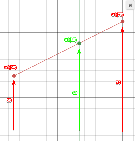
A visual representation of linear interpolation.

Marginal values are normalised to bound U(o) in the interval [0,1].

We want to find a value function U that is compatible with our preference relation ≻.
I know what you’re thinking: now we’ve fully set everything up, we can convert this into a linear programming problem.
What? You weren’t thinking that?
Don’t be scared; it looks ugly at first, but I’ll guide you through it.
First of all, the value function U(o) is compatible if it satisfies the following constraints:

There's no way I’m typing all that.

Constraints, hmm? That sounds like an LP problem...
This is what this looks like as an LP problem:

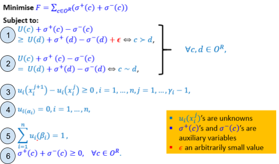
There’s sigmas and epsilons and aaaargh
Don’t worry, I’ll go through each new thing, and each constraint.

The epsilon is just some arbitrary small number. It’s not a variable we’re finding a value of; it can be any tiny number, like 0.0001 or something.
This is to make sure the first constraint works like a strict inequality, so our LP problem doesn’t find trivial solutions we don’t want. Remember, LPs can’t have strict inequalities, so we need to “make” one with a non-strict inequality and a smol epsilon value.
The sigmas represent how much error there is. We’re making the assumption that these are additive value functions, but they might not be. σ+ and σ- represents how far “off” we are, either too high or too low, respectively.
The values (breakpoints) are the unknowns we’re trying to figure out. That’s why we split them up into subintervals: so we can calculate this function in discrete steps by finding breakpoints.

... and now, the constraints:

This constraint makes sure that when U(c) ≥ U(d), that also means c ≻ d.
This constraint makes sure that when U(c) = U(d), that also means c ∼ d.
This constraint makes sure that any breakpoint is always bigger than its preceding one, so e.g. makes sure that u1(75) is bigger than u1(50).
This constraint makes sure that the breakpoint of the worst finite evaluation is always 0 (in other words, the breakpoints always start at 0).
This constraint ensures that ui’s are chosen so that U is normalised.
This constraint defines the range of the error values (0 or greater).

We’re minimising the sum of our errors.

If the error sum is non-zero, then our solution is not compatible.
If the error sum is zero, there is no error, so our solution is compatible (there exists at least one value function that is compatible).

Here, we’re assuming that ui is an additive value function, so we don’t really need the sigmas here.

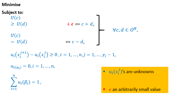
Ahh, much cleaner!
If you’re still super confused, then here’s the main thing to take away:

We got a partial preference relation on a subset of outcomes.
We want to look for a value function U that is compatible with that partial preference relation, and map out a full preference ordering using it.
We split the ui functions into subintervals with discrete breakpoints.
We use LP to find those breakpoints such that U is compatible with the partial preference relation.
We use the breakpoints to get the value function U, and use it to map out a full preference ordering.

If the optimal value of the objective function (error sum) is greater than zero, consider:

Increasing γi (number of subintervals)
Revising the preference ordering on OR.

UTAGMS - Robust Ordinal Regression

UTA is cool, but there are limitations:

We pick any random compatible value functions, if they exist. Isn’t that a bit wasteful?
Marginal value functions are piecewise linear, and you arbitrarily pick the number of subintervals.
Complete preference ordering is needed on reference outcomes (the ordering you start off with).

Basically, UTA sucks.
You should be using the c h a d UTAGMS, and here’s why:

Takes into account the whole set of compatible additive value functions
Marginal functions are general non-decreasing functions (no more weird piecewise stuff)
Reference outcome ranking does not need to be complete

There are some assumptions we need to make first.

The agent knows their partial preference over the set of reference outcomes .
ui’s are normalised to bound U(o) in the interval [0,1].
gi’s are known, and their range is bounded.

Now that we have that out the way, let’s introduce what UTAGMS actually calculates for you.
For any , we can ask:

Are and ranked the same way across all compatible value functions?
Is there at least one compatible value function that ranks as least as good as ?

When we apply this to all pairs , we get:

Necessary weak preference relation ≽N

a ≽N b ⇔ U(a) ≥ U(b) for all compatible value functions
Basically, when we say a ≽N b, then this is true for every single possible compatible value function we could calculate.

Possible weak preference relation ≽P

a ≽P b ⇔ U(a) ≥ U(b) for at least one compatible value function
Basically, when we say a ≽P b, then this is true for at least one possible compatible value function that we could potentially calculate.

From the partial preference ordering, for any :

a ≽ b ⇒ a ≽N b

If is at least as good as in the reference outcomes, then it’s trivial that all the value functions we’re going to calculate will satisfy that too (because we’re using the reference outcomes as a base).

a ≻ b ⇒ not(b ≽P a)

If is strictly better than in the reference outcomes, then there isn’t going to be any value functions we’ll find where is at least as good as .

So basically, the value functions we’re going to calculate will have the same orderings as the partial preference orderings from the reference outcomes.

The way UTAGMS computes compatible value functions is similar to UTA, but with a slight difference.
First, I should introduce :

is the permutation on the set of indices of outcomes from OR that reorders them according to the increasing evaluation on attribute i.
Makes no sense? No problem.
In other words, it gets the index of the outcomes, in the order of the specified attribute, in order of increasing evaluation (lowest to highest).
Here’s an example using sweetness (i = 1) from the ice cream table all the way up:

gi(strawberry) = 70
gi(vanilla) = 60
gi(chocolate) = 40

gi(a𝝉i(1)) <= gi(a𝝉i(2)) <= gi(a𝝉i(3))
gi(chocolate) <= gi(vanilla) <= gi(strawberry)

𝝉i(1) would point to chocolate, because it has the lowest sweetness.
𝝉i(2) would point to vanilla, because it has the next lowest sweetness after chocolate.
𝝉i(3) would point to strawberry, because it has the highest sweetness.

Now that I have that out the way, here are the constraints that a compatible value function must follow:

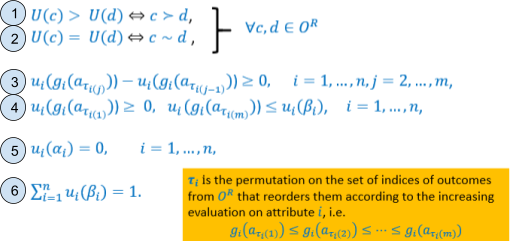
Let’s go over each constraint and explain it:

When U(c) > U(d), then also c ≻ d
When U(c) = U(d), then also c ∼ d
The marginal value of an outcome, with respect to an issue, should be greater than the marginal value of another outcome, given that the evaluation of the first outcome is greater than that of the second. E.g. given that gi(strawberry) = 70 and gi(vanilla) = 60, this checks that ui(gi(strawberry)) ≥ uigi(vanilla)).
This checks the range of the marginal values of outcomes. It checks that the marginal value of the outcome with the smallest evaluation doesn’t go below 0, and that the marginal value of the outcome with the biggest evaluation isn’t above the maximum.
This sets the minimum marginal value to 0.
This is here to normalise the value function U.

For some weird reason, this set of constraints is called . I’ll just call it EAR.

Save your breath asking me, I have no idea why it’s called that.

Not even the slides explain.

So how do we convert EAR into an LP problem and get the compatible value functions?
You can do the same thing we did in UTA, and add a small epsilon value to the first constraint.
If the LP is infeasible, then there is no compatible value function.
This can happen because:

Agent’s preferences do not match the additive model
Agent has made an error in their statements

Alongside compatible value functions, we can also compute ≽N and ≽P.
We need to define something first, though.
For all pairs of outcomes , let be pretty much the same as , except it orders the set , and let .

Now, the characteristic points are evaluation values that start from the minimum and ends at the maximum, and in-between are the evaluation values of each outcome in increasing order.
Here’s an example:

Let’s say and are mint choc chip and bubblegum, and also that:
gi(mint choc chip) = 55
gi(bubblegum) = 65
Remember that the range of sweetness evaluation is [0,100].
Therefore the characteristic points are:
gi0 = 0
gi1 = gi(chocolate) = 40
gi2 = gi(mint choc chip) = 55
gi3 = gi(vanilla) = 60
gi4 = gi(bubblegum) = 65
gi5 = gi(strawberry) = 70
gi6 = 100

With that out of the way, we can define the set of constraints E(a,b):

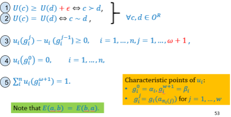
We’re going to use this to compute ≽N and ≽P, but let’s look at each constraint:

When U(c) > U(d), then also c ≻ d
When U(c) = U(d), then also c ∼ d
The marginal value of one characteristic point is greater than the marginal value of the characteristic point that came before it. For example, say gi(strawberry) = 70 and gi(bubblegum) = 65, this constraint checks that ui(strawberry) ≥ ui(bubblegum).
The marginal value of the smallest characteristic point should be 0.
This is here to normalise the value function U.

Alright, so what? We have this set of constraints, but we’re not doing anything with it yet.
Here’s why:

For a given pair :
To calculate ≽N, minimise U(a) - U(b) with subject to E(a,b).
To calculate ≽P, maximise U(a) - U(b) with subject to E(a,b).
If our solution is non-negative, then a ≽N or P b.

How does this work?

If a ≽ b, then surely U(a) ≥ U(b), right?
And if U(a) ≥ U(b), then U(a) - U(b) ≥ 0.
Remember that U(a) - U(b) is our objective function.
That means if we find a solution that is non-negative, then a ≽N b or a ≽P b or whatever, must be true, for our given solution.

But why minimise / maximise?

For ≽N, when we minimise, we are finding the smallest possible difference between U(a) and U(b) while still being non-negative.
If we find that the smallest difference between U(a) and U(b) throughout all compatible value functions is non-negative, then that means all other differences between U(a) and U(b) throughout all other compatible value functions must also be non-negative.
Therefore a ≽ b must be true for all compatible value functions, and therefore a ≽N b.
For ≽P, we want to find any compatible value function where this difference is non-negative.
We’re effectively increasing our chances of finding one by maximising, because we’re trying to get the largest possible difference that’s closest to a non-negative value.
When the difference is non-negative, we know that there exists one compatible value function where a ≽ b is true, because we’re sitting on one: the solution we’ve arrived at. Therefore, a ≽P b.

For each pair of outcomes , we perform 4 LPs to establish:

a ≽N b
b ≽N a
a ≽P b
b ≽P a

However, we may not need to perform all 4 at times, given that:

≽N implies ≽P

The result of the first two LPs can decide whether or not we perform the last two.

Once we calculate ≽N and ≽P , we give these to the agent, so they can use it to:

extend their preference information
decide on the next elicitation steps.

Auctions

So far, we’ve only seen negotiations as a way of resolving conflicts between agents.
However, as mentioned before, there’s two more:

Auctions
Voting

In this section, as you’ve probably guessed, we’re looking at auctions!

An auction is a way of allocating scarce resources.
There’s many types of auctions with different properties, but they all share the same things:

Should maximise social welfare (allocate resources to the one who values them most, e.g. highest bidder)
Should be individually rational (agents should not be worse off from participating)
Should not be manipulatable (agents are incentivised to behave truthfully)
Should maximise revenue (if applicable).

Suppose we are selling a single item. Just one item. I don’t know, a chair or something.

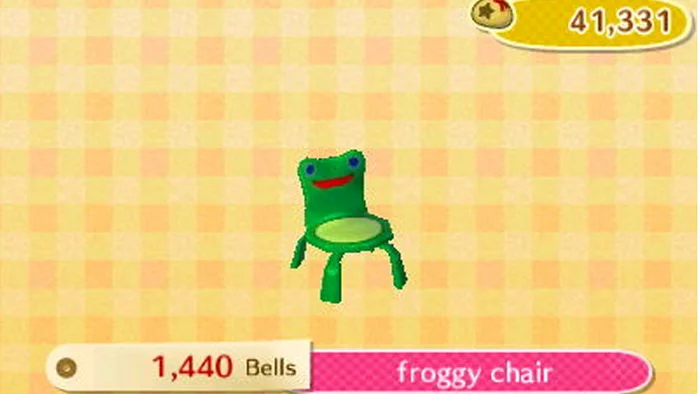
I’m auctioning off a froggy chair.

There’s different families of auctions for this:

Open-outcry auctions:

English auction
Dutch auction
Japanese auction

Sealed-bid auctions:

First-price auction
Second-price (a.k.a Vickrey) auction
All-pay auction

Which is better? There’s only one way to find out...

Let’s set the stage a little and define single-item auctions some more.

A seller has a single item, e.g. a froggy chair.
There exists ‘n’ strategic bidders.
Each bidder ‘i’ has a private valuation (or willingness to pay). We’ll call this .
Our bidder utility model is a quasilinear utility model.

If ‘i’ loses, and has to pay pi, their utility is -pi.
If ‘i’ loses, and doesn’t have to pay, their utility is 0.
If ‘i’ wins, and has to pay pi, their utility is θi - pi.

We’re assuming:

Independent private value model (valuation does not depend on other bidders’ valuation)
Bidders cannot collude

To decide who wins, we need an allocation rule + a payment rule.

The goal of an auction is to maximise social welfare.
We can define social welfare like this:

xi is 1 if ‘i’ wins, and ‘0’ if ‘i’ loses.
Only one bidder can win, so out of all bidders, only one has xi = 1, and the rest has xi = 0.
In a single-item auction, maximising social welfare means awarding the item to the highest bidder.
That’s our allocation rule: pick the bidder whose bid is the highest.

Now we need a payment rule. Ooh. That’s where things get interesting.

Types of auctions

Let’s have a look at all these other auctions and see what their payment rules are:


English auction: Auctioneer starts at a low “reservation price” Bidders shout ascending prices, with some minimum increment set by the auctioneer. Auction ends once bidders stop bidding Highest bidder wins the item and pays their bid.	Dutch auction: Auctioneer starts at a high bidding price Auctioneer lowers the price until someone bids The item is allocated to the first bidder at that current price

Sealed-bid auction: Each bidder submits a bit in a sealed envelope Bidders do not see each other’s bids Bids are collected by the auctioneer The auctioneer determines the winner and the price to pay This depends on the type of sealed-bid auction. In first-price sealed-bid auction, the highest bidder wins and pays the price they bidded.	Vickrey (second-price sealed-bid) auction: A type of sealed-bid auction where the highest bidder wins, but they pay the second highest bid (or reserve price, whichever is higher). Named after William Vickery.

Analysing Auctions

How do we analyse auctions?
In other words, how do we reason with them? Mathematically?
Let’s start converting an auction into a game:

Let denote the bid placed by bidder .
Let denote the bid profile of all bidders (basically, a tuple of everyone’s bids)
The set of all actions available to each bidder is all possible bids that they can place.

If a bid is valid, any bidder is allowed to place it.

The utility of each bidder depends on:

their private valuation or type , as well as
the outcome (allocation + payment), which in turn depends on and the bids placed by other bidders ().

Auctions are not strategic-form games.
However, if there are enough assumptions (all bidders know each other’s preferences, there are two bidders etc.) you can treat it like one to answer questions about the auction, such as Nash Equilibrium.
Auctions are actually Bayesian games.
This module doesn’t go into detail about Bayesian games, but if you’re doing Algorithmic Game Theory with me next semester, you’ll learn all about them!

Alongside Bayesian games, we’ll also be covering FNAF theories.

Alright, so we’ve given names to everything.
To actually start calculating stuff, we need a decision theoretic framework.
A decision theoretic framework gives bidders beliefs about the bid distribution, and allows us to calculate things such as the chance that a bid will be the highest out of everyone.

We can assume that in ties, the bidder loses, so the tie-breaking rule is not in our favour (unless the question says otherwise).
Let’s say that F(b) denotes the probability that all other bids are less than b. That means F(b) is the probability that b is the winning bid, with no ties.

Our goal is to find a winning strategy of the form

Where is the set of actions or bids, which maximises the expected utility for any valuation .
So we want to give this function our valuation (which could be how high we’re willing to bid or something), and we want it to spit out the best actions we can take.

First-price auction expected utility

The utility of a valuation in a first-price auction is given by:

if (if bi is the winning bid)
otherwise (if bi is the losing bid)

The expected utility given bid bi is then:

The syntax is basically saying “the utility of valuation θi given that we’re doing bid bi”. Think of it like the conditional probability syntax of Bayesian.
Just think of this like a function that takes two arguments:

To find the optimal bids, you calculate the expected utility for all possible bids.
However, you can cut out some bids that you know will be useless (e.g. bids higher than your valuation will always yield negative utilities).

What? You want an example?
Dude, it’s 3am as I’m typing this...
... but that’s no problem! You’re worth making examples for :D

Let’s say I’m auctioning my froggy chair, and that you can only bid between £1 - £5, in £1 increments, and the probabilities are:

F(0) = 0 (if you bid nothing, it’s certain that others will bid higher)
F(1) = 0.3
F(2) = 0.6
F(3) = 0.7
F(4) = 0.95
F(5) = 1.0 (if you bid £5, it’s certain that nobody’s gonna bid that high)

... and let’s say that θi = 4.
There’s no point calculating the expected utility for bi = 0 because that’s basically losing, or bi = 5 because that’s above our valuation.
So we’ll calculate the range of 1 to 4:

E[ui(4) | 1] = (4 - 1)F(1) = 3 * 0.3 = 0.9
E[ui(4) | 2] = (4 - 2)F(2) = 2 * 0.6 = 1.2
E[ui(4) | 3] = (4 - 3)F(3) = 1 * 0.7 = 0.7
E[ui(4) | 4] = (4 - 4)F(4) = 0 * 0.95 = 0

As you can see, you get the highest expected utility when bi = 2, so you should pick that one.

Now, the slides go on to explain about continuous bid distributions, but it says we don’t need that for the exam, so I won’t go too far into it.
All I’ll say is that:

it uses the derivative of F
you find the optimal bid by setting the derivative to 0 (finding the turning point of F)
if you have a uniform distribution for F, you should always bid half of your valuation.

Vickrey Auction: Discrete bids expected utility

For Vickrey auctions, it’s a little more complicated.
Remember that with Vickrey, we pay the amount of the second highest bid.
That means the utility of a valuation is given by:

if (if bi is the winning bid)
otherwise (if bi is the losing bid)

In English, this means that if we have the winning bid, our utility is our valuation minus the value of the second highest bid.

Let:

... denote the probability that the highest opponent bid is exactly .
Why?

Remember that F(b) means “probability that all other bids are less than b with no ties”.
So means “probability that all other bids are less than b + 1”.
That also means “probability that second highest bid / highest opponent bid can be up to b”.
So the whole formula means:

“probability that highest opponent bid can be up to b - probability that highest opponent bid can be up to b - 1”

Intuitively, you can kind of see how this results in “probability that highest opponent bid is exactly b”.

Then the expected utility of bid bi is:

English please?

The first part, , is the expected value you gain if you win.
The second part, , is the “payment”; it’s the estimated “second highest bid” value that you have to pay.

Vickrey Auction: Continuous bids expected utility

When we have a Vickrey Auction with continuous bids instead of discrete bids, we use an integral instead of a sum.
Then the expected utility of bid bi is:

If you’re wondering why the integral is from 0 to bi, that’s because the upper bound should be the largest opponent bid at which bi will still win. That means the largest opponent bid should be bi - ε, where ε is infinitesimally small.
If ε is so small it’s practically zero, we can just use bi as the upper bound.

With discrete bids, finding the optimal bid is easy: we just calculate the expected utility for all the reasonable bids we can make.
But for continuous bids, it’s not that simple. If we tried that here, we’d have infinitely many bids to calculate through!
That’s why, to find the optimal bid, we find the bid that makes the derivative of the expected utility equal to zero.
We do this because when the derivative of the expected utility is zero, that’s the expected utility’s “turning point”, meaning at that point, the bid will be at its maximum.

The optimal bid is given by:

Wait... if the derivative = 0 simplifies to that, and then you divide on both sides, then you get .
That’s right; in Vickrey auctions, your valuation is always your optimal bid.
That means our strategy is always .
In layman’s terms, if you come across a Vickrey auction, it’s always best to just bid the maximum of how much you’re willing to pay straight away.

Strategy-proofness

A strategy is weakly dominant if, no matter what any of the other parties do, that strategy will get you the same (if not higher) utility than any other strategy.

In the Vickrey auction, is a weakly dominant strategy.

An auction is called truthful if you can adopt a strategy that is weakly dominant.
Other names include strategy-proof, and incentive-compatible in dominant strategies.

A good way to visualise this is to prove that the Vickrey auction is truthful.
To prove that it’s truthful, we need to prove that is a weakly dominant strategy.
To prove that, we need to show that every other strategy yields the same utility.
We can do this by several cases:

We win

We lose

We bid higher than

Equal utility

We still win, and pay the same amount.

Lower utility

We either lose and pay nothing, or win but pay more than our valuation (negative utility).

We bid lower than

Lower utility

We either win and pay the same amount, or lose and get nothing.

Equal utility

We still lose and pay nothing.

In any case, bidding truthfully maximises our utility.

How about Dutch auctions?
Here, is the point at which you bid when the clock reaches the value (assuming nobody has bid before).
So what’s our optimal strategy here?
Again, it’s . I’ll tell you why:

If , you’ll pay greater than your valuation.
If , someone else is likely to win, and pay a price that’s well within your valuation, even though they were willing to pay less than you (a.k.a the item had more value to you than them)

It’s the same in first-price sealed-bid auctions.
You don’t gain any new information until the winner is announced, so you might as well bid your valuation.
This is true for both first-price sealed-bid auctions and Dutch auctions.
Because they have identical optimal strategies, they are strategically equivalent.

Things are a bit different in an English auction.
Let’s say that strategy ‘si’ means that you don’t bid any higher than that value.
It doesn’t mean you bid si straight away, it means that every bid bi ≤ si (in other words, you should not bid past this point)
In an English auction, the optimal strategy is si = .

So, in a Vickrey auction, you bid your valuation.
In an English auction, you don’t bid past your valuation.
It’s not the same, but it’s similar. This is called weakly strategically equivalent.

There are questions that these frameworks cannot answer:

Individual rationality: which auctions ensure that agents are not worse off from participating?
Manipulation: which auctions incentivise truthful behaviour?
Efficiency: does the item always go to the agent who values it the most?
Revenue: which auction creates more revenue for the seller?

Bayes-Nash Framework

Remember when I talked about Bayesian games and I made that dumb Game Theory joke?
This is kinda about that.

In the independent private value model (the one we’ve been using up till now), player utility is based on their own individual valuation and the bids of others, not the valuations of others, because they don’t know them.
However, agents do have a prior distribution over players’ profiles, which is common knowledge.
In other words, every agent knows of a distribution of valuations that applies to each player, so we can make very educated guesses over other players’ possible valuations.
This is what makes an auction a Bayesian game.
The solution concept for this is a Bayes-Nash equilibrium (BNE), but we won’t go into that right now.

Revenue Equivalence

Formal:

Assume that all bidders are risk-neutral and utility maximisers, and each has an independent private valuation for the single item, drawn from a common cumulative distribution F(θ) that is strictly increasing and atomless on [L, H]. Then any auction mechanism in which

in equilibrium, the item will be allocated to the agent with the highest valuation, and
any agent with valuation L has an expected utility of zero...

... yields the same expected revenue, and hence results in any bidder with valuation θ making the same expected payment.

Alright, before you roast me for copy-pasting the slides, let me put this into layman’s terms.
Two auctions are revenue equivalent when in both auctions, if a player wins by bidding x amount in auction 1 and bidding the same amount in auction 2, the estimated amount paid by the highest bidder is the same, no matter which auction you use.

The four single-item auctions are all revenue equivalent.
This includes:

English auction
Dutch auction
First-price sealed-bid auction
Vickrey auction (second-price sealed-bid)

This is called the Revenue Equivalence Theorem.
There’s proofs I’ve found online, but they’re long and complicated.

Trading Agents

There are automatic bots that bid in auctions, you know.
They bid on stuff like:

Online auctions such as eBay
Financial exchanges (algorithmic trading)
Betting exchanges
Online advertising auctions

If you feel like procrastinating,

here’s a Drawception I found about robot auctioneers.

There’s also auctions selling off advertising space, too.

Sponsored search: allocation of ad space alongside search results.

Multiple slots on a single page sold simultaneously.
Uses an auction called Generalised Second Price (GSP) Auction.
For a while it was thought that GSP is a “proper” generalisation of Vickrey and is strategy-proof; but it has been shown that it is not!
Bidding and auction fully automated.

Banner Advertising: advertising on regular web pages usually auctioned off.

Auctions are run by ad exchanges such as DoubleClick and Facebook Exchange (FBX).
Each item is a slot on a webpage.
Auctioned off individually using the Vickrey auction.

Wasn’t that interesting?
What?! You found it boring?
Sorry. I write the notes, but I don’t write the slides.
Here’s another cute robot auctioneer to make up for it:

Here’s one that’s not so cute:

Voting

We’ve looked at auctions and the algorithms for them.
Now, we’ll look at voting!

Social choice theory (or voting theory) is the study of a class of protocols for making group decisions.
If you’ve never spoken to a human being before, voting is when a group of agents come to a single agreement and pick one outcome over a set of many.
This affects all agents (i.e it is a social outcome).
Some examples could be:

When and where to meet?
Who should execute this task?
Which JoJo’s Bizarre Adventure part is the best?

and everyone’s favourite...

Which flavour ice-cream should we pick?

If you don’t like this example, then you won’t like the rest of this section.

Obviously, everyone has different opinions over ice-cream flavours.
You might prefer strawberry over chocolate, whereas your friend might prefer chocolate over strawberry, but Jerry might prefer vanilla over all of them.
These are called their preferences.
We can’t pick everyone’s favourite, because they’re all different. We can only pick one.
Therefore, we need to combine these preferences to derive a social outcome.
The main mechanism in which we achieve this is through voting.

I’ve droned on about what voting is, but let’s define things more formally.
Let be the set of agents (or voters).
Each agent will have their own preferences over a set of outcomes (or candidates): . This is like our set of ice-cream flavours.

If we have , we have a pairwise election.
If we have , we have a general voting scenario.

Let be the set of all preference orderings over (this would contain all the different preferences you could possibly have for ice-cream flavours).
Let be a preference ordering for agent (for example, if agent 2 preferred vanilla over bubblegum, then vanilla bubblegum would be true).
We denote as any preference ordering profile, i.e. or where it is multiplied times (this would contain a single combination of all the different possible preferences of every single agent).

The Social Choice Problem

So we have everyone’s preferences. How do we combine them into a choice?
First, let’s define what we want:

A social welfare function takes voters’ preferences and returns a social preference order (an aggregated preference).

For example, strawberry vanilla chocolate

A social choice function takes voters’ preferences and returns a single choice.

For example, strawberry

Let refer to the outcome of a social welfare function.
Given a preference ordering profile and a social welfare function , then is called the aggregate ranking for .

So we’ve defined our mathematical voting “framework”, but how do these social functions work?
What are some voting procedures / systems?
There’s different ways to aggregate preferences, and we’ll go over a few. Let’s define an example first.

You go to Sprinkles, with 14 other people. There is a world shortage of ice-cream, so you can only pick one scoop of one flavour to share. Each voter has a numerical ID, and a numerical preference shown on the right, with 1 being the preferred option and 3 being the least preferred. For voter 1, their preference would be: strawberry vanilla chocolate	Voter	Strawberry	Vanilla	Chocolate
	1	1	2	3
	2	1	2	3
	3	1	2	3
	4	1	2	3
	5	1	2	3
	6	1	2	3
	7	3	2	1
	8	3	2	1
	9	3	2	1
	10	3	2	1
	11	3	2	1
	12	3	2	1
	13	2	3	1
	14	2	1	3
	15	2	1	3

Plurality Vote

The first voting function we’ll go over is the Plurality Vote.
Basically, you rank each outcome based on how many times it’s the most preferred option.

Strawberry is preferred 6 times
Vanilla is preferred 2 times
Chocolate is preferred 7 times

According to Plurality Vote, chocolate is the winner.
However, even though it’s preferred by 6, 8 others prefer something else!
By majority, they don’t want chocolate, but something else. Something’s not right...

This is an example of the Condorcet Paradox!
This means that sometimes, there are scenarios where no matter what we pick, a majority of voters will be unhappy.
Here’s a more succinct example:

Phoenix: strawberry vanilla chocolate
Miles: vanilla chocolate strawberry
Larry: chocolate vanilla strawberry

No matter which ice cream flavour we pick, a majority (⅔) of the boys won’t get their favourite.

A Condorcet winner is the candidate who always wins in pairwise elections using plurality.
In other words, it’s the option that, when put in one-on-one votes against other options, our winner will always come out on top.
In our example, if strawberry won the elections strawberry vs chocolate and strawberry vs vanilla, then strawberry would be a Condorcet winner.
An option like this doesn’t always exist (like in our examples using Plurality).

A voting system satisfies the Condorcet criterion, if it always chooses a Condorcet winner when one exists.
Rules (voting systems) satisfying this property are called Condorcet methods and are said to be Condorcet consistent.

Let’s give another example. Who is the Condorcet winner in our Sprinkles example?
Let’s do all combinations of pairwise elections:

Strawberry vs Vanilla: 7 , 8 ‎
Strawberry vs Chocolate: 8 , 7 ‎
Vanilla vs Chocolate: 8 , 7 ‎

Vanilla always wins in pairwise elections, so therefore vanilla is the Condorcet winner here.

Copeland Method

Here’s a method that is Condorcet consistent, is within the Condorcet methods, and satisfies the Condorcet criterion (that all means the same thing, by the way).
In the Copeland method, outcomes are ranked based on their pairwise victories minus their pairwise losses.
Pretty simple, right? Plus, it’s easy to see why it’s Condorcet consistent.
Let’s use the Copeland method on our Sprinkles example:

Strawberry vs Vanilla: Vanilla wins ‎
Strawberry vs Chocolate: Strawberry wins ‎
Vanilla vs Chocolate: Vanilla wins

Now, to calculate everyone’s scores:

Vanilla: 2 wins - 0 losses = 2
Strawberry: 1 win - 1 loss = 0
Chocolate: 0 wins - 2 losses = - 2

So our Copeland ranking goes vanilla strawberry chocolate.
It seems like vanilla is our Copeland winner, and as we’ve seen before, it’s also our Condorcet winner. Nice!

This method also works when there isn’t a Condorcet winner.
There’s an example in the slides if you want, but there’s nothing new.

Borda Count

With this voting system, we take into account all information from a preference order.
The Borda count gives a score for every outcome based on a sum of how highly it was ranked by each voter.
More specifically, it goes like this:

With outcomes, for each voter, the first choice is awarded points, the second choice is awarded points, and so on.
For example, voter 1 likes strawberry the best, so a score of 3 is added to strawberry. They like vanilla next, so a score of 2 is added to vanilla, and they like chocolate last, so a score of 1 is added to chocolate.
This is done for all voters, and the scores of the outcomes are summed, and those scores are used for the final social preference order.

In our example, the Borda counts are:

Strawberry has 30 points
Vanilla has 31 points
Chocolate has 29 points

So, using Borda count, our order would be vanilla strawberry chocolate.

That looks pretty Condorcet to me!
... right?
Even though it’s the same result as Copeland, which is Condorcet consistent, Borda count is not Condorcet consistent.
You want an example this time?
Here; I’ve put how many points each outcome gets in brackets.

Voter	Strawberry	Vanilla	Chocolate
1	1 (3)	2 (2)	3 (1)
2	1 (3)	2 (2)	3 (1)
3	1 (3)	2 (2)	3 (1)
4	3 (1)	1 (3)	2 (2)
5	3 (1)	1 (3)	2 (2)
Borda count	11	12	7

The Condorcet winner here is strawberry, because the majority (3 out of 5) prefers strawberry, so trivially, strawberry will win all pairwise elections.
However, according to the Borda count below, the Borda winner is vanilla.
Yikes...

Properties of voting procedures

So we’ve covered some concrete examples of voting procedures.
Let’s talk a little more generally now.

Given a voting procedure, how do we know that it’s... you know... good?
And not crap?
First of all, we need to know what “good” is.
We need to define some desirable properties of voting systems that can be satisfiable.

Social Welfare Functions

What are some desirable properties of social welfare functions?
Remember, these are the ones that return a preference, not a single outcome.
Here’s three:

Pareto Efficiency

A social welfare function is Pareto efficient if, whenever every agent prefers over , then .
In other words, if every agent prefers vanilla over chocolate, in one way or another, then the social preference order (the outcome preference) should rank vanilla higher than chocolate.

Independence of Irrelevant Alternatives (IIA)

A social welfare function is independent of irrelevant alternatives if whether is ranked above in the social outcome depends only on the relative orderings of and in agents’ preferences.
In other words, let’s say we have an election of strawberry, vanilla, chocolate, and mint choc chip. If the social preference order ranks strawberry over vanilla (strawberry vanilla), then the voters’ preferences of strawberry against vanilla should be the only preference that affects that outcome ranking.
If the voters all preferred chocolate to mint choc chip, and then suddenly changed their mind to prefer mint choc chip to chocolate, neither of those would affect the strawberry over vanilla ranking in the social preference order, because only the voters’ preferences of strawberry and vanilla can do that.
Strawberry and vanilla are independent of irrelevant alternatives; namely, chocolate and mint choc chip.

Non-dictatorship

A social welfare function is non-dictatorial whenever there is no voter such that for all , if then .
In other words, if a voting system is non-dictatorial, there can never be a situation where it’s up to a single voter to make the deciding vote.
Have you ever had a vote amongst friends where your vote is last, but there is the same number of votes for each option, making your vote the deciding vote?
In a situation like that, you are the dictator, because your choice will directly determine the outcome.
If a voting system does not satisfy non-dictatorship, we call it dictatorial.

Arrow’s Theorem: For elections with more than 2 candidates, any social welfare function satisfying Pareto efficiency and IIA are dictatorial.
In other words, if we have Pareto efficiency and IIA, we can’t have non-dictatorship.
This means we can’t have every one of these properties in one voting system.
We can have up to two, maximum, like the CAP theorem.

Social Choice Functions

What are the desirable properties of social choice functions?
Remember, these are the ones that return a single option, not a preference.
Here’s three:

Weak Pareto Efficiency

A social choice function is weakly Pareto efficient if, when every agent prefers over , then cannot be the outcome of the social choice function.
This is like Pareto efficiency with social welfare functions, except it only applies to the most preferred option in our social preference order; in other words, our output choice. That’s why this is called “weak”.
For example, if every voter prefers vanilla over strawberry, then strawberry cannot be the output choice.

Monotonicity

A social choice function is monotonic if, for every preference profile , such that , if is another profile such that whenever for every agent and every alternative , then as well.
In other words, if you have a preference profile with an output choice of chocolate, and you have some other preference profile with voters who have the same preferences of chocolate strawberry/vanilla, then that “other” preference profile should have an output of chocolate.

This is a little hard to visualise, so let’s use an example.
Let’s say we have our first preference profile:

Phoenix: strawberry vanilla chocolate mint choc chip
Miles: vanilla strawberry mint choc chip chocolate
Larry: chocolate mint choc chip strawberry vanilla

... and according to our social choice function, the selected choice is strawberry.
Now, let’s say we have our second preference profile:

Apollo: strawberry mint choc chip vanilla chocolate
Trucy: vanilla strawberry chocolate mint choc chip
Athena: mint choc chip chocolate strawberry vanilla

If our social choice function satisfies monotonicity, it would also select strawberry for our second preference profile.
Why?
Informally, because strawberry is always in the same place, comparing the first profile and the second profile (strawberry is Phoenix and Apollo’s first choice, Miles and Trucy’s second choice etc.). First profile’s choice is strawberry, so because of this, it should be the second profile’s choice too.
Formally, because the voters in the second profile pick strawberry something whenever the voters in the first profile pick the very same strawberry something, where that “something” is every alternative option, like vanilla, chocolate etc.

Non-dictatorship

A social choice function is non-dictatorial if there does not exist an agent such that always selects the top choice in ’s preference ordering.
It’s pretty much the same as the social welfare function version: there should never be a situation that leaves one voter with the deciding vote.

Muller-Satterthwaite’s Theorem: For elections with more than 2 candidates, any social choice function satisfying weak Pareto efficiency and monotonicity is dictatorial.
In other words, if we’ve got weak Pareto efficiency and monotonicity, we can’t have non-dictatorship.
This is just like Arrow’s theorem! We can’t have all three, but only two, maximum.

Hmm...
What if we could manipulate the vote to get a better outcome?
Let’s say our preference is strawberry vanilla chocolate, and chocolate is the chosen option.
What if we changed our preference to get a better outcome? Like, instead of making strawberry our preferred option, we make vanilla our preferred option, to try and get a result of vanilla, which our profile likes better than chocolate?
We would be misrepresenting our preferences to the voting procedure.
If we’re able to do that in some way, that makes our social choice function manipulable.

More formally, the social choice function is manipulable if, for some preference ordering profile:

... and voter , there exists some such that

In a manipulable voting system,

it’s possible to lie to get a better outcome.

That’s bad! We don’t want liars; we want things to be fair.
Can we come up with a voting procedure that is not manipulable?

Gibbard-Satterthwaitte’s Theorem: Any social choice function with at least three outcomes that satisfy citizen sovereignty and is truthful (i.e. non-manipulable) is dictatorial.

Citizen sovereignty: for every outcome , there exists a preference profile such that the social choice function returns .
In other words, it’s possible for any outcome to be the chosen outcome, depending on the voters. There aren’t any outcomes in which it’s impossible for that to be the chosen outcome, no matter what the votes say.
For example, a voting system that always picks ‘strawberry’ does not satisfy citizen sovereignty, despite it being non-manipulable and non-dictatorial.

So, yes, we can come up with non-manipulable voting systems, but it’s very likely that it’s going to be dictatorial.
In addition, manipulating elections is pretty hard:

There are loads of unknowns, like other voters’ preferences, whether they’re being manipulative too etc.
Computing a “lie” can be costly, depending on the voting protocol used