Evolution of Complexity
Matthew Barnes
Recorded Lectures 3
Introduction 5
Evolutionary Algorithms 6
Representation of Individuals 8
Fitness Function 8
Selection 9
Variation Operators 11
Variations on a theme 13
Evolution History 14
Pre-Darwinian Evolution 14
Natural Selection 15
The Modern Synthesis 18
Fitness Landscapes 19
Definitions 19
Intuition 21
Properties 22
Epistasis 23
Examples: Synthetic Landscapes 25
Functions of unitation 25
NK landscapes 25
Royal Roads and Staircases 28
Long paths 29
Examples: Biological Landscapes 31
Complications 32
Sex 36
Linkage Equilibrium 37
Fisher / Muller Hypothesis 40
Muller’s Ratchet 41
Crossover in EAs 42
Focussing Variation 42
Schemata and Building Blocks 46
Schemata Theorem 46
Building Block Hypothesis 46
Two-Module Model 48
Coevolution 51
Pairwise vs Diffuse 53
Sasaki & Godfray Model 54
Coevolution in GAs 55
Why use Coevolution 57
Problems with Coevolution 59
Cooperative Coevolution 60
What is Cooperative Coevolution 61
Competitive vs Cooperative 61
Divide and Conquer 63
Modularity 64
Types of modularity 64
Concepts of modularity 66
Examples 67
Simon’s “nearly-decomposable” systems 67
Modularity in EC 70
Hierarchical IFF as a Dynamic Landscape 71
Representations 76
Graphs (TSP) 77
Structured Representations 80
Variable-size Parameter Sets 81
Trees 82
Grammar Based Representations 83
Cellular Encoding 84
Turtle Graphics 85
Advanced Representations 86
Artificial Life 89
Concept, Motivation, Definitions 89
Examples 90
Karl Sims Creatures 90
Framsticks 91
Darwin Pond 91
Cellular Automata Based 92
Computer Program Based 94
Arrow of Complexity 95
Information Entropy 95
Kolmogorov Complexity 95
Structural Complexity 96
McShea’s Passive Diffusion Model 97
Hierarchical Structure 99
Natural Induction (not examinable) 101
Compositional Evolution 108
Gradual vs Compositional 110
Complex Systems 112
HIFF 113
Random Genetic Map and SEAM 114
Recorded Lectures
-
At the time of writing this, it’s tricky to find the
recorded lectures for a given topic.
-
Therefore, I compiled this table.
|
Week
num (date)
|
Monday 9AM
|
Monday 11AM
|
Tuesday 1PM
|
|
1 (1/2)
|
Richard had really bad connection
problems.
|
Richard forgot to record.
|
Evolutionary Algorithms part 1
-
Assignment 1
-
Hillclimber
-
Four requirements for natural
selection
-
Evolutionary Algorithms (EAs)
-
Pseudocode of EA
-
Components of EA
-
Representation
-
Fitness functions
-
Selection (roulette wheel)
|
|
2 (8/2)
|
Evolutionary Algorithms part 2
-
Boltzmann
-
Stochastic Universal Sampling
-
Tournament
-
Truncation
-
Rank-based
-
Steady state vs generational
|
Evolutionary Algorithms part 3
-
EA schools
-
Parameters of EAs
-
Assignment 1
|
Evolution History part 1
-
Levels of life
-
Carolus Linnaeus’ “Systema
Naturae” 1735
-
Early Evolutionary Theory
-
Lamarck
-
Pre-Darwinian Views
-
Voyage of the Beagle
-
Natural Selection
-
Darwin’s “On the Origins of
Species”
-
Trouble with Inheritance
-
Post-Darwin
|
|
3 (15/2)
|
Evolution History part 2
-
Questions on evolution history
-
The Modern Synthesis
-
Neo-Darwinism
-
Fisher vs Wright
-
Contention over
‘speciation’
-
Punctuated Evolution
|
Evolution History part 3 and Fitness
Landscapes part 1
-
Contention over ‘level of
selection’
-
Growing knowledge
|
Fitness Landscapes part 2
-
Definition
-
Wright’s genotype sequence
space
-
Wright’s fitness landscape
-
Properties of landscapes
-
Epistasis
-
Synthetic landscapes (unitation)
|
|
4 (22/2)
|
Fitness Landscapes part 3
-
Epistasis networks
-
NK-landscapes
-
Royal Road / Staircase
-
Path lengths
-
Probing high-dimensional landscapes
-
Fitness distance scatter plots
|
Fitness Landscapes part 4
-
Biological examples
-
Visualisations
-
Protein folding
-
“And then it gets
complicated...”
-
Individuals vs Populations
-
Neighbourhoods and variations
-
Designing a landscape
|
Assignment 1 solution
-
Richard’s results of Assignment
1
-
GAs vs hillclimbers
|
|
5 (1/3)
|
|
Sex part 1
-
Two-fold cost of sex
-
Sexual reproduction
-
Sexual recombination
-
Crossover
-
Genetic linkage
-
Linkage (dis)equilibrium
|
Assignment 2
-
Assignment 2 explanation
-
Reading through papers
|
|
6 (8/3)
|
Sex part 2
-
Fisher/Muller hypothesis
-
Muller’s Ratchet
|
Sex part 3 and Crossover in EAs part 1
-
Doesn’t go over deterministic
mutation hypothesis
-
Sex from POV of an EC
-
Natural Selection and Variation study and
review
-
“Focussing search”
-
Hurdles problem
-
Schemata and building blocks
|
Crossover in EAs part 2
-
Schemata and building blocks
-
GA vs hillclimber on RRs
-
Two-module model
-
Richard’s weird PDF simulation
|
|
7 (15/3)
|
Crossover in EAs part 3 and Coevolution
part 1
-
Analysis with + without recombination
-
Analysis mutation-only vs crossover
-
Definition of coevolution
-
Normal vs reciprocal
-
Pairwise and diffuse coevolution
-
Sasaki & Godfray model
-
Coevolutionary algorithm basics
-
Why use them
|
Coevolution part 2
-
Why use them
-
Coevolution examples
-
Funny YouTube video of evolved 3D
creatures
-
Subjective vs objective fitness
-
Types of coevolutionary failure
-
Cool Java simulation animation
|
Cooperative Coevolution
-
Cooperative coevolution
-
Shared domain model
-
Divide and conquer
-
Talking about papers from Assignment
2
|
|
🐰 EASTER 🥚
|
-
Types of modularity
-
Concepts of modularity
-
Simon’s
“nearly-decomposable” systems +
examples
-
Modularity in EC
-
Hierarchical IFF
-
Genotype → phenotype →
fitness
-
Types of representation
-
Structured genotypes
-
Tree encodings
-
Grammar-based encodings
-
Turning strings into structure
-
Strong / Weak
-
Wet / Dry
-
Sims creatures, Framsticks
-
Darwin Pond
-
Cellular automata based
-
Computer program based
-
Information Entropy
-
Kolmogorov complexity
-
Structural complexity (object, process,
(non)hierarchical)
-
McShea’s passive diffusion
model
-
Hierarchical structure
-
Major transitions in evolution
-
(Not examinable; tbh I barely understand
this lecture)
-
Motivation
-
What is Natural Induction
-
Examples
-
Gradual vs Compositional
-
Complex systems
-
HIFF
-
Genetic maps
-
SEAM
|
|
|
|
|
Introduction
-
Hi there! 👋
-
Welcome to the Evolution of Complexity Notes.
-
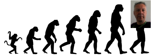
In case you didn’t realise, I’m human!
-
I am the result of hundreds of millions of years of
evolution and natural selection.
-
If you’re not a screen-reader, then you are,
too.
-
Sure, you might look like your parents, but if we go really
far back, we’ll find some things that look nothing
like you.
-
Like really small protein compounds from the primordial
soup.
-
But enough about soup. Let’s compare you with a
calculator.
|

|

|
|
A calculator
(one that you’re allowed to use in
exams)
|
You, probably
|
-
Hmm... yes... that’s definitely a calculator, and
that’s definitely a person.
-
What’s the difference?
-
One is engineered; designed by us, and (if engineered properly) composed of modular components, with low coupling and
high cohesion.
-
The other is living; designed by nature, with loads of
tightly-packed organs that are very highly coupled.
-
What I’m trying to say here is that evolved things
are very complex.
-
We want to make our own things that are this complex.
-
Hence, we have evolutionary algorithms!
-
With it, we can make things like this neural net that plays snake.
-
Evolution by natural selection is the best explanation we
have for the complexity of living things.
-
But remember, that’s just a theory. A ga- uh, a scientific theory.
-
It’s not perfect, and it’s your duty as a
scientist to find holes in it....
-
... or, just do what the lecturers tell you and get decent
marks.
Evolutionary Algorithms
-
Do you remember stochastic local search?
-
If not, here’s a refresher on hill-climbing:
-
Start with a random solution
-
Make a small change to it
-
If that change was better, keep it. If not, discard.
-
Repeat until we reach a solution we like
-
It’s an algorithm used to search a solution space and
find a local maximum.

A computer scientist climbing a solution space
to its maximum using a stochastic local search algorithm.
-
This is kind of like evolution, right?
-
There’s generations, and mutations, and stuff like
that.
-
Evolutionary algorithms (EA) are like hill-climbers, but with a population.
-
Some individuals in the population might be luckier than
others.
-
We need to concentrate on those, so their children can
survive, and “discard” the others.
-
It sounds cruel, but that’s nature.
-
There are four requirements for evolution by natural selection:
- Reproduction
-
Individuals can replicate themselves.
-
Copy(A) → B
- Heritability
-
Offspring is similar to their parents.
-
B ≈ A
- Variation
-
There are differences, or “mutations”, in
children.
-
Vary(Copy(A)) → B1, B2, B3
-
B1 ≠ B2 ≠ B3
-
Change in fitness
-
The variations cause our fitness to change.
-
Copy(A) → B
-
Fitness(A) ≠ Fitness(B)
-
Here is the outline of an evolutionary algorithm (EA):
-
Initialise all individuals of a population
-
Until (satisfied or no further improvement)
-
Evaluate all individuals
For i=1 to P; Quality(Pop[i]) → Fitness[i]; End
-
Reproduce with variation
For i=1 to P;
Pick individual j with probability proportional to
fitness
Pop2[i] =
Pop[j];
Pop2[i] =
mutate(Pop2[i]);
End
Pop2 → Pop;
-
Output best individual
-
The necessary components of an EA are:
-
Representation of individuals
-
Fitness function
- Selection
-
Variation operators
-
Let’s go through each one.
Representation of Individuals
-
As a computer scientist, you know that computers store
information as data.
-
That means, to represent our individuals, we need to encode
them into data.
-
There are many ways to do this:
|
Problem
|
Individual encoding
|
|
A function that takes 20 binary
arguments.
Maximise the function.
|
A 20-bit binary number
e.g. 00101110101000010111
|
|
A graph theory problem, like TSP
|
A string of node names, making a path
e.g. BHGADCEF
|
|
Where to place x number of items
|
A set of (x,y) coordinates
e.g. (12,34), (56,78), (90,12)
|
-
As you can see, there’s loads of ways to encode
individuals as data.
-
If we can encode an individual into data, and we can copy data...
-
... that means we can copy an individual.
-
That covers our reproduction requirement of natural selection!
Fitness Function
-
In evolution, each individual has fitness.
-
That means we need a fitness function that takes an
individual and returns a fitness.
-
Our fitness function needs to directly correlate to our
“goal”, or what we want to achieve out of our
algorithm.
-
That way, when we maximise our fitness, we’re closer
to achieving our goal.
- For example:
|
🤔 Problem
|
🏁 Goal
|
💪 Fitness function
|
|
A function that takes 20 binary
arguments.
Maximise the function.
|
We want to find a set of arguments that
maximises our function.
|
The value outputted by the function.
|
|
Travelling Salesperson Problem (TSP)
|
Travel all nodes in the shortest length
|
Length of the tour
(we would have to minimise our fitness function
in this case, e.g. make it a cost
function)
|
|
Position of drilling sites on an oil
field
|
We want to extract as much oil as we can.
|
Oil yield from a simulation of the oil
field.
|
An individual with a high fitness.
Selection
-
How do we select what individuals to, uh...
“mate” and pass on to the next generation?
-
There’s a variety of ways to pick.
-
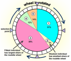
One of these ways is using fitness proportionate selection (FPS).
-
The slides compare it to a roulette wheel, but it’s
basically individuals with a higher fitness have a higher
chance of being selected.
-
For example, if we had a population of 2, and #1 had a
fitness of 6, and #2 had a fitness of 4, then we’d
have a 60% chance of selecting #1 and a 40% chance of
selecting #2.

-
Another way is Boltzmann Selection: a more refined version of the fitness proportionate
selection above.
-
The formula goes like this, where
 is the probability of picking individual
  :
:
 ,
,
-
 - the fitness function of individual
-
 - standard deviation in distribution of fitness
-
 controls selection
-
 means weak (neutral) selection; all individuals have an equal
chance
means weak (neutral) selection; all individuals have an equal
chance
-
 means strong (choose the fittest) selection; only the highest
fitness will be picked
means strong (choose the fittest) selection; only the highest
fitness will be picked
-
Yet another way is Stochastic Universal Sampling (SUS).
-
Where FPS chooses several solutions from the population by
repeated random sampling, SUS uses a single random value to
sample all of the solutions by choosing them at evenly spaced intervals (source).
-
Comparing it to the roulette wheel, FPS spins the wheel
multiple times to get samples.
-
However, SUS has multiple, evenly-spaced pointers on the
wheel, and the wheel is spun once.
-
What’s good about this is that weaker individuals
have a chance to reproduce too, and the fittest members
won’t saturate the candidate space.
-
In other words, there’s less variation in the number
of offspring any one individual has.
-
Huh? You want even more selection operators?
-
Fine. Here’s three more:
-
Pick
 individuals, and choose the individual with the
highest fitness
individuals, and choose the individual with the
highest fitness
-
Pick any individual in the top half of the population
-
Assign a rank to each individual based on fitness (e.g. worst fitness has rank 1)
-
Pick an individual with probability proportional to rank (or 1/rank, if that’s what you need).
-
How is this different from FPS?
-
In rank-based selection, only the ordinal assignment of fitness matters, not cardinal (it only matters that fitness is greater; not how much
by).
-
For example, say i1 has a fitness of 1, and i2 has a fitness of 2.
-
i1 would have rank 1, and i2 would have rank 2.
-
FPS and rank-based selection wouldn’t be any
different.
-
Now, what would happen if i2 had a fitness of 2,000?
-
FPS would pick i2 waaaay more times over i1!
-
However, their ranks are still equal, so the probabilities
of rank-based selection wouldn’t change.
Variation Operators
-
There are two main variation operators. One of which is mutation.
-
With mutation, we slightly change the properties of an
individual.
-
How much we change by is completely random. Some might
change a lot, and some might not change at all.
-
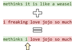
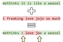
For example, we could mutate the sentence “methinks
it is like a weasel” by going through each letter and
changing it to a different letter under a probability of
1/28 (28 being the number of letters in the sentence).
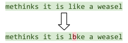
-
Therefore, on average, we only change 1 letter per
mutation, but it’s still possible for some sentences
to change a lot and some to not change at all.
-
How volatile our mutations can be (mutation rate) is a set variable for our evolutionary algorithm that
we can change. We can tweak it to maximise the performance
of our algorithm.
Polydactyly; a rare mutation in humans
that gives us more than 5 fingers / toes.
-
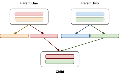
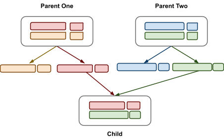
The other kind of variation is crossover, or recombination.
-
This refers to using information from two or more
individuals to make a brand new individual.
-
There’s three versions of this:
-
Randomly select one point on the strain.
-
Everything above the point is from parent 1, and everything
below the point is from parent 2.
-
Randomly select two points on the strain.
-
Everything to the left of the first point and to the right
of the second point is from parent 1, and everything between
the first and second points are from parent 2.
-
Randomly select genes from parent 1 and 2 with even
probabilities for each.
-
Here is the outline of our evolutionary algorithm 2.0, with crossover:
-
Initialise all individuals of a population
-
Until (satisfied or no further improvement)
-
Evaluate all individuals
For i=1 to P; Quality(Pop[i]) → Fitness[i]; End
-
Reproduce with variation
For i=1 to P;
Pick individual j with probability proportional to
quality
Pick individual k with probability proportional to
quality
Pop2[i] =
crossover(Pop[j],Pop[k]);
Pop2[i] =
mutate(Pop2[i]);
End
Pop2 → Pop;
-
Output best individual
Variations on a theme
-
There are two main kinds of genetic algorithm:
-
Offspring replaces one person of the population each time
they are generated
-
Pick parents for reproduction
-
Generate offspring with variation
-
Put offspring back into population
-
For each generation, P offspring are generated for the next
population
-
Pick parents for reproduction
-
Generate offspring with variation
-
Put offspring into NEW population
-
Current population = new population
-
For some weird reason, academics like to argue about
evolutionary algorithms.
-
So much so that they split into factions, or
“evolutionary algorithm schools”.
-
Here’s a range of evolutionary algorithm
schools:
-
Binary representation
-
Crossover is important
-
ES: evolutionary strategies
-
Real-valued representations
-
No crossover
-
Evolved mutation rate
-
For evolving programs
-
Specifically, LISP s-expressions
-
EP: evolutionary programming
-
Finite state automata
-
Mutation only
-
According to Richard, the schools GA, ES, and EP came
together to form their own conference, but the one in charge
of GP said no and continued doing their own thing.
-
Setting the parameters of an evolutionary algorithm is
something of a black art.
-
There’s:
-
If it’s too big, you waste computation
-
If it’s too small, there’s no useful
diversity
-
Mutation rate / crossover rate
-
If it’s too low, there’s not enough
innovation
-
If it’s too high, there’s too much
destruction
-
Choosing a good fitness function
-
Selection pressure
-
Fitness scaling via: Boltzmann selection, rank-based,
tournament size, truncation fraction
-
Diversity maintenance methods
Evolution History
-
Nowadays, evolution and natural selection are pretty
well-known and generally accepted.
-
But how did we get here? This section covers the history of
evolution up to this point.
Pre-Darwinian Evolution
1735
-
Carolus Linnaeus published Systema Naturae.

-
It was a book that described all living things that Carolus
had studied, and put them into categories, like animals and
plants.
1758
-
Carolus Linnaeus published the 10th edition of Systema Naturae.
-
It set up the formal classifications that are used (with few changes) today.
-
With that, systematic biology took off (finding living things and figuring out what kind of a
thing it is in Linnaeus’ book).
1785
-
James Hutton published Theory of the Earth, or an Investigation of the Laws
Observable in the Composition, Dissolution and Restoration
of Land upon the Globe.
Around 1800
-
Jean-Baptiste Lamarck put forward the theory of inheritance of acquired characteristics, or “Lamarckism”.
-
He did not see all life sharing a common ancestral
tree.
-
An early proponent of evolution was Charles Darwin’s
grandfather, Erasmus Darwin.
-
The main two problems back then was:
- Religion
-
How can evolution create such complex organisms?
-
“Natural theology”, advocated by the likes of
William Paley, used complexity of life as evidence for
God.
1830
-
Charles Lyell published Principles of Geology.
-
The Biblical view of creation is starting to turn
over.
-
The world is far older than traditionally believed.
Natural Selection
1831
-
Darwin sailed out on The Beagle (a boat).
-
He publishes The Voyage of the Beagle.
-
It raised questions which lead to the theory of natural
selection.
-
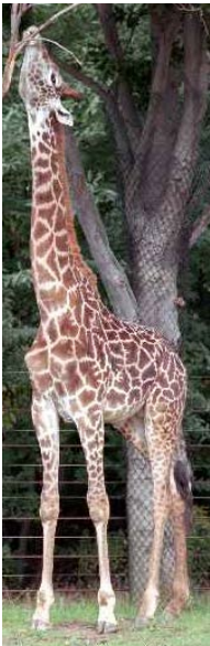
When he came back, he had examined a collection of
finches.
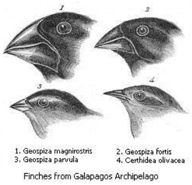
-
He thought they were all one species, but they proved to be
many species.
-
The simplest explanation was that a single migrant had adapted to the habitat on different islands.
-
He came up with a mechanistic explanation: natural selection:
“Natural variations in populations that provide
small
selective advantages will take over the
population.”
-
It was strongly influenced by Thomas Malthus’ Essay on the Principle of Population (1798).
-
Darwin then spent the next 20 years collecting
evidence.
-
During this, he published definitive work on cirripedes (marine invertebrates including barnacles).
-
Another naturalist, Alfred Wallace, who also thought
Malthis was cool, arrived at the same theory of natural
selection.
-
He was also inspired by Darwin’s Voyages of the Beagle. He had explored South America and Malaya.
-
After the last trip, he sent his ideas to his mentor,
Charles Darwin.
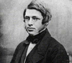
-
Wallace agreed to publish jointly with Darwin.
1832
-
Darwin wrote On the Origins of Species.
-
Everyone accepted the theory of evolution because:
-
Darwin was popular
-
He had 20 years worth of evidence
-
He had a lot of arguments, including:
-
power of artificial selection by human breeders
-
population of isolated islands by chance migrations
-
relatedness of species in a tree like structure
-
He also addressed problems with evolution:
-
missing fossil record
-
difficulty of evolving complex structures (e.g. the eye)
-
People believed evolution, but not natural selection.
-
They didn’t think it could make complex
structures.
-
Darwin wrote six editions of Origins of Species, the final editions accepting possibilities of mechanisms
besides natural selection.
-
Darwin could never explain inheritance.
-
His problem was:
-
Under crossover, any variation should be averaged
out.
-
How can there be enough variation for natural selection to
work?
-
Gregor Mendel had the answer with his Experiments in Plant Hybridization (1865) (the theory of discrete genetics), but it was neglected until 1900.
|
|
Darwin’s Problem
|
|
|
|
Let’s say we have a population of tall
and short people.
When a tall person and a short person have a
kid, under reproductive crossover, that kid will
be medium height.
After a while, the population of tall and short
people will average out to medium people.
With that, how will there be enough variation
in the population to achieve natural
selection?
(Of course, this isn’t how genetics
works, but they didn’t know that.)
|
|
-
Everyone was stuck arguing about natural selection for the
next 70-100 years.
1882
-
After Darwin died, advocates for natural selection shut up
for a bit.
-
Lamarck’s theory of “acquired
characteristics” was revived.
-
They came up with another theory:
-
Large mutations called “saltations” produce
dramatic changes to organism structure, which explains
speciation.
-
This contrasted the gradual, small changes of conventional
Darwinism.
-
When Mendelian genetics was rediscovered in 1900, it was
seen as a blow to natural selection.
-
Basically, natural selection was on the ropes.
-
It took three young Turks to turn things around...
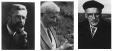
The three young Turks who turned things around.
-
Ronald A Fisher
-
Sewell Wright
-
John B S Haldane
-
They read the Origin of Species and ignored the establishment thinking.
-
They said “wait... what if:
-
Natural selection occurs
-
and genetic inheritance occurs”
-
And thus, the modern synthesis was born.
The Modern Synthesis
A cool picture from Wikipedia illustrating modern
synthesis
1930
-
Fisher wrote the book The Genetical Theory of Natural Selection.
-
It didn’t catch on until around 17 years later.
-
Haldane helped push these ideas into mainstream
biology.
1960
-
Natural selection and the modern synthesis, often called neo-Darwinism, triumphed.
-
But people still argued.
-
Fisher and Wright argued.
-
Wright said inbreeding is important, and small populations
were necessary to explore complex fitness landscapes.
-
People also argued about what causes speciation.
-
Saltationists put this down to large mutations.
-
Geographical isolation was considered one of the major
causes of speciation.
-
Ernst Mayr says that speciation by isolation is one of the
driving forces of invention by evolution (and says that small populations in peripheral locations
are more likely to be sources of innovation).
1972
-
Eldedge and Gould proposed the theory of punctuated evolution.
-
This is evolution that consists of periods of rapid
evolution in speciation events, followed by long periods of
stasis.
-
It explains rapid changes found in the fossil record.
-
People also argue about what level selection operates
at.
-
Richard Dawkin and his fanbase say it’s only at the
gene level.
-
But it may be more than that... who knows?
Fitness Landscapes
Definitions
-
Genome / Chromosome: A vector / string of genes
-
e.g. a bit string
-
“001111”
-
Gene: one variable in a genome
-
Allele: The value of a gene
-
‘tall’, ‘blue’, 0, 1, A, a
-
Locus: The position of a gene in a genome
-
The locus of ‘e’ is further from
‘a’ in “abcde”
-
Genotype: A type of genome
-
The difference between a genome and a genotype is that
genomes refer to each individual string of genes, and
genotypes refer to what the genome represents (the
semantic).
-
For example, in the population:
-
0001111
-
0001111
- 1001000
-
1100011
-
There are 4 genomes, but 3 genotypes.
-
A fitness landscape consists of:
-
A set of genotypes
-
A neighbourhood
-
We arrange genotypes in a space such that:
-
Similar genotypes are close
-
Different genotypes are far
-
e.g. neighbouring genotypes differ by a single allele
-
Height of surface in this space = Fitness of each
genotype
-
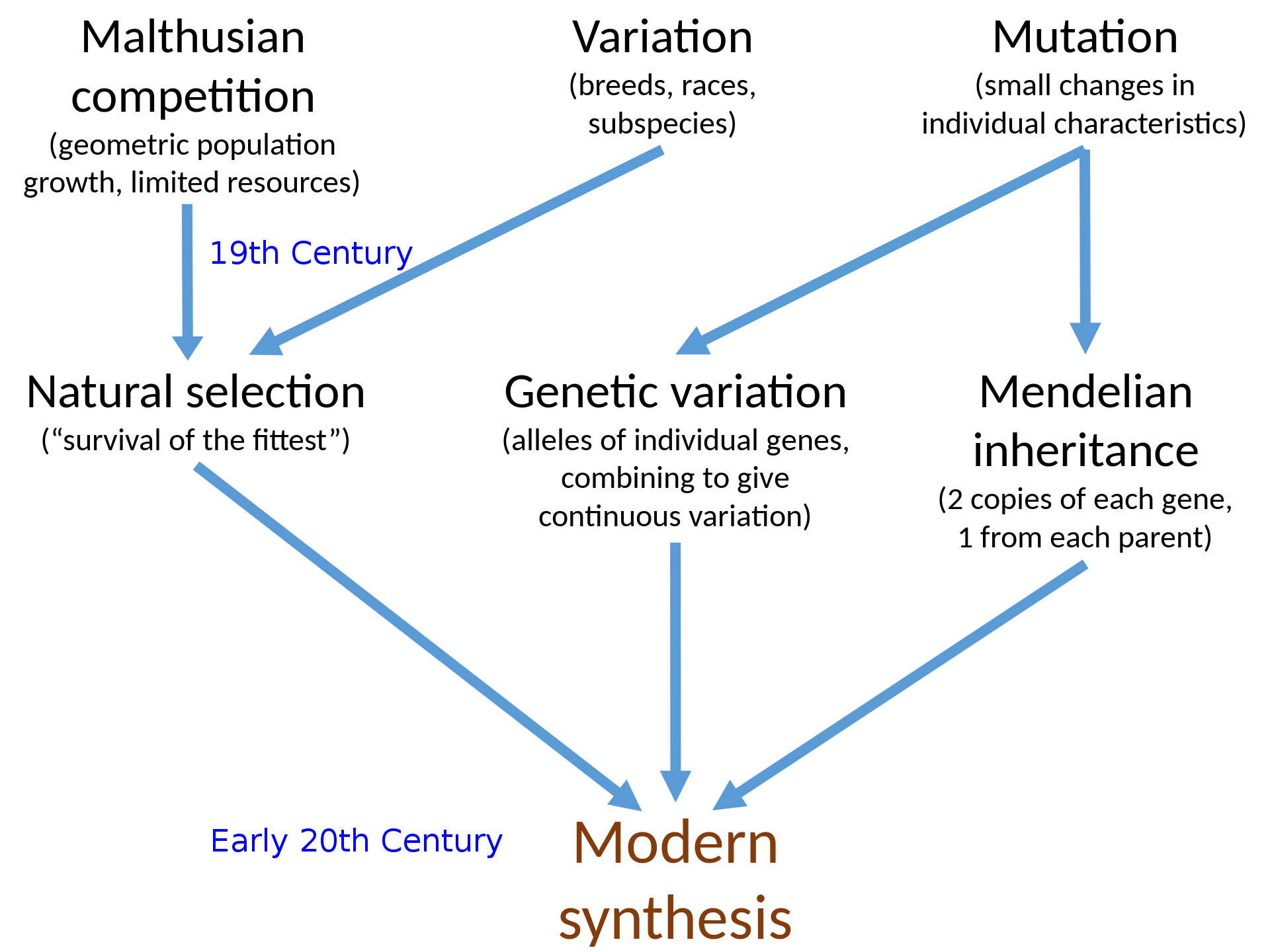
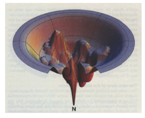
By rendering a fitness landscape in a graph, we can
visualise how changes in the genome affect fitness.
-
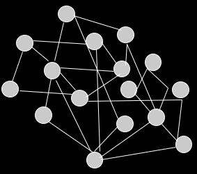
Here’s an example of a fitness landscape:
-
As you can see, some genotypes do not yield good fitness,
and some yield really good fitness.
-
There are also hills that a population can climb to achieve
better fitness.
-
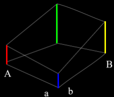
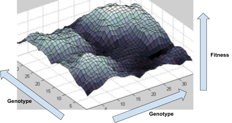
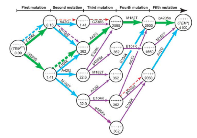
Wright’s genotype sequence space is a representational DAG (directed acyclic graph) of all the different genotype sequences, and how they
relate to each other.
-
Here’s a few examples:
-
These graphs go from left to right, and map out every
possible derivable genome.
-
Each node represents a possible derived genome.
-
Each edge adds one new gene at a time.
-
The distance from each node represents the number of
genetic changes to reach from the source genome to the
destination genome.
-
The number of genes represent the number of dimensions a
genotype sequence space has.
-
Alright, these Crystal Maze looking things are cool, but
with lots of genes, there’s going to be lots of
dimensions.
-
It’ll become really hard to visualise with lots of
dimensions.
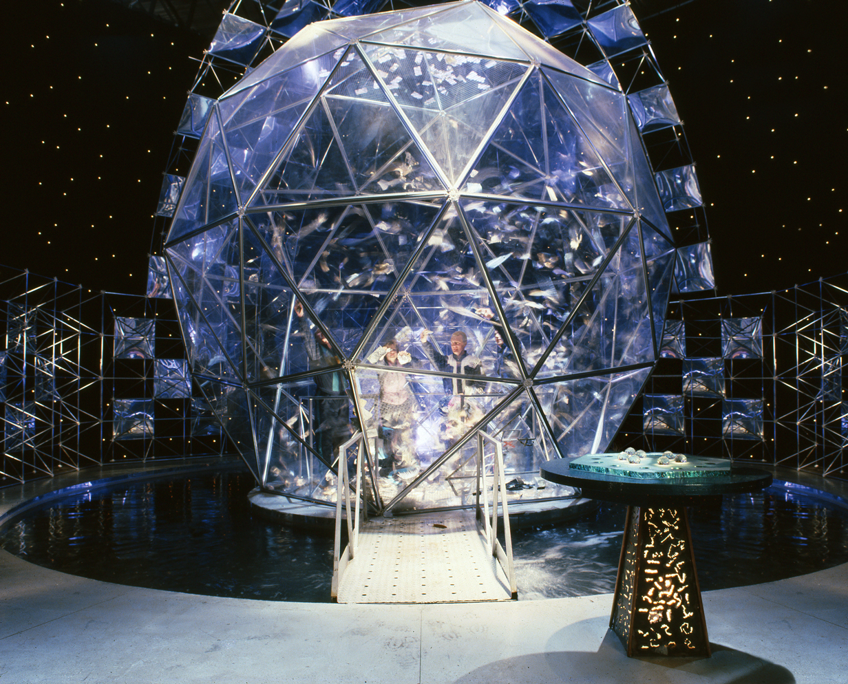
An IRL genotype sequence space, with people inside it.
-
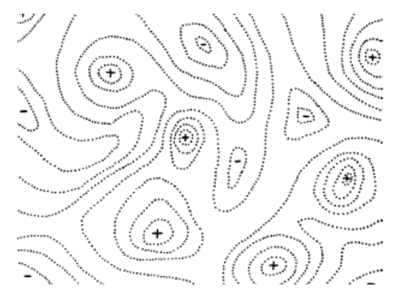
Wright’s fitness landscape is like a normal fitness landscape, but represented
with contours instead of a fancy 3D graph:
-
The contours represent fitness elevation in a
two-dimensional fitness landscape.
-
The +’s represent peaks in fitness, and the -’s
represent valleys in fitness.
Intuition
-
We said before that evolutionary algorithms are like
hillclimbers, but with a population.
-
But how does that actually change anything?
-
Let’s have an example:
-
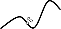
With hillclimbing, we have a single individual and we
“climb up the hill” we are currently sitting on,
in the fitness landscape.
-
But look! Just to the right of us, there’s an even
higher hill.
-
Because hillclimbing only cares about the hill we’re
on, we’ll miss the chance to get an even better
maximum.
-
Because evolutionary algorithms have a population, and in
that population we have diversity, we can go up different
hills.
-
The higher hill has greater fitness than the lower hill, so
the population going up the higher hill will eventually be
favoured.
-
That doesn’t mean we’ll always get the best
maximum though: at the start, the subset that is going up
the taller hill could die out faster than the subset going
up the smaller hill, giving us the smaller maximum
again.
Properties
-
Fitness landscapes have several properties:
-
How similar neighbouring points are in terms of
fitness
-
How “rough” or “spiky” the fitness
landscape surface looks
-
Local optima, global optima
-
Global optima is the very highest fitness peak in the
landscape.
-
Local optima are peaks, but not the highest peaks.
-
How likely is it I arrive at a particular optimum?
-
In other words, how likely, if I started from somewhere on
the space, would I end up at this optimum?
-
If the spike has a greater base width, then it’s more
likely that a random space would land on that spike.
-
So it also refers to the base width of the spike at the
bottom.
-
Neutrality and redundant mappings
-
Is the gradient zero?
-
In other words, is the fitness landscape elevation
completely flat?
-
If so, then all the surrounding genotypes map to the same
fitness value.
-
This is also called a neutral plateau.
-
Paths of (monotonically) increasing fitness
-
Do I need to go down in fitness and cross a ‘fitness
valley’?
-
One of the biggest problems of all stochastic local search
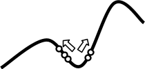
methods is going from one peak to another (typically a higher peak).
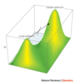
-
In this two-peak fitness landscape, if we’re stuck at
the local optimum, how can we reach the global
optimum?
-
This is a problem with natural evolution in biology,
too.
Epistasis
-
Gross... that’s not what I meant!
-
Let’s look at the next definition:
-
Uh... how about I just tell you instead?
-
Epistasis: the fitness effect of an allele depending on the genetic
context of that allele.
-
It creates ruggedness in a fitness landscape.
- Huh?
-
In other words, the change in fitness due to substituting
one allele for another at one locus, is sensitive to the
alleles that are present at other loci.
-
You can think of epistasis as the property of genes having
“dependencies” on each other.
- What?
-
Let me just show you an example instead...
Examples: Synthetic Landscapes
-
There are two kinds of landscapes:
-
Artificial landscapes we design ourselves, for
demonstration and testing purposes
-
Fitness landscapes based on real-world data
-
First, we’re going to look at some synthetic
landscapes.
-
There’s many different kinds...
Functions of unitation
-
The name means ‘from many dimensions to
one’.
-
One of these functions include counting the number of
1’s in a bitstring:
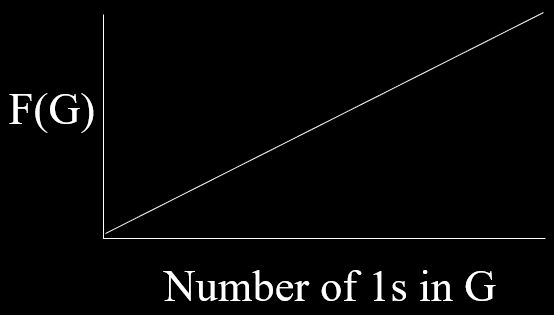
-
This is very similar to our “methinks it is like a
weasel” coursework.
-
You can also tweak this slightly to make a “trap
function”:
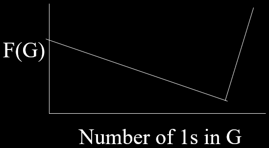
-
By having this fitness valley, it’s a great landscape
to test EAs on.
NK landscapes
-
Before we go over NK landscapes, we need to cover epistasis
networks.
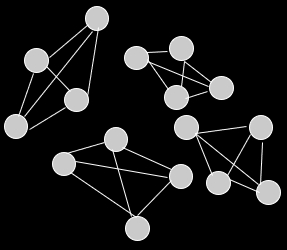
-
An epistasis network is a graph that represents the epistasis in a
genome.
-
The nodes represent the problem variables (or genes).
-
The edges represent dependencies / epistasis between
variables.
-
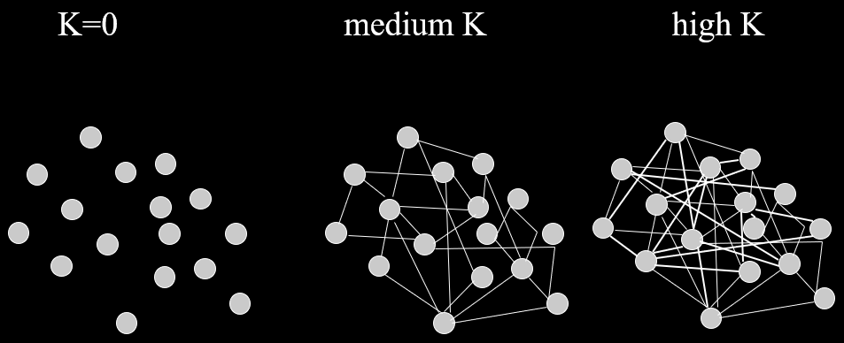
An NK landscape is a fitness landscape with epistasis, with
two variables controlling the level of epistasis:
-
 - number of variables
-
 - number of dependencies between variables
-
In other words, each variable has a fitness contribution
that is a function of its own state and others.
|
Example: NK landscapes are Kim Jong-un’s favourite
fitness landscape
|
-
We have this genome, and it’s got
epistasis, where:
|
1
|
2
|
3
|
4
|
5
|
6
|
7
|
8
|
|
0
|
1
|
1
|
1
|
0
|
0
|
1
|
1
|
-
So that means each gene also depends on
three other genes for their fitness.
-
The dependencies between genes are
represented by colour.
-
As a graph, that looks like this:
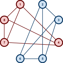
|
-
When
 , there are no dependencies.
-
The landscape looks like one big mountain, like Mt.
Fuji.
-
As increases, the landscape gets more rugged; more peaks
in a smaller space.
Royal Roads and Staircases
-
Royal Roads split the variables into sub-systems / groups /
blocks, so the fitness only goes up if a whole sub-system is
completed.
-
You can think of royal roads as special kinds of NK
landscapes, where the dependencies are in adjacent
groups.
-
Here’s an example with a couple of genomes with the
counting 1’s:
|
Bit string
|
Fitness
|
|
1111 0000 0000 0000
|
8
|
|
0000 1111 0000 0000
|
8
|
|
0000 0000 1111 0000
|
8
|
|
0000 0000 0000 1111
|
8
|
|
1111 1111 0000 0000
|
16
|
|
0000 0000 1111 1111
|
16
|
|
1111 0000 1111 1111
|
24
|
|
1111 1111 1111 1111
|
32
|
-
The epistasis networks of royal roads have clear
separations between the groups:
-
With royal roads, you can solve any of the groups in any
order.
-
But with royal staircases, you must solve them in a certain
order.
-
A royal staircase is a special kind of royal road where a completed
block only contributes fitness if the blocks before it are
all completed also.
-
Here’s another example with counting 1’s:
|
Bit string
|
Fitness
|
|
1111 0000 0000 0000
|
8
|
|
1111 1111 0000 0000
|
16
|
|
1111 1111 1111 0000
|
24
|
|
1111 1111 1111 1111
|
32
|
|
0000 1111 0000 0000
|
0
|
|
0000 0000 1111 0000
|
0
|
|
1111 0000 1111 1111
|
8
|
|
1111 1111 0000 1111
|
16
|
-
Why are they called royal staircases?
-
It’s because their fitness landscapes look like
stairs.

-
Each fitness “step” is a neutral plateau.
-
Going from one neutral plateau to the next is called
“portal genotypes”.
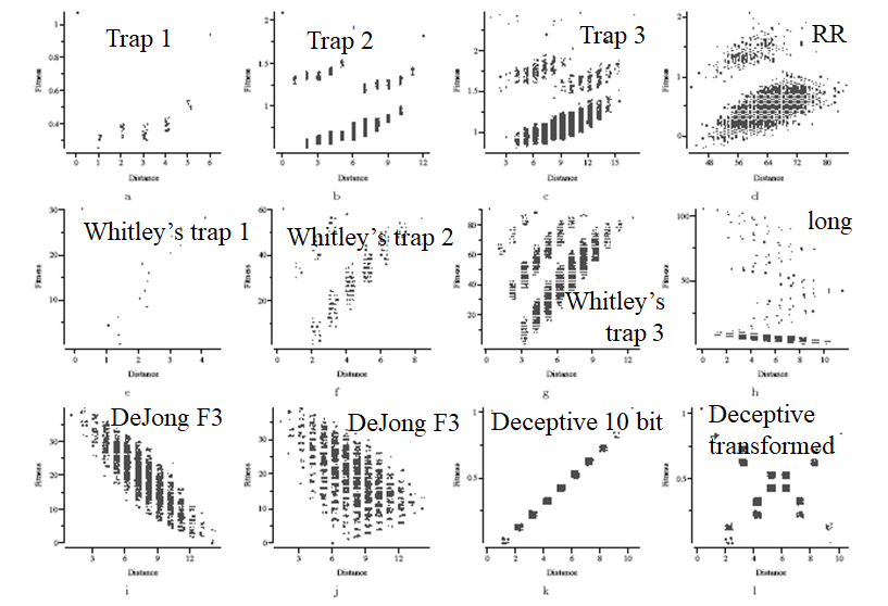
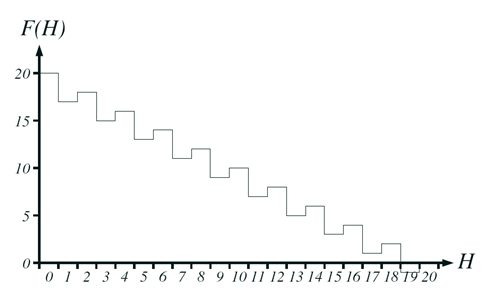
Long paths
-
An adaptive walk is the path a population takes from a point on the
fitness landscape up to a peak, where fitness is highest for
that hill.
-
What’s the longest an adaptive walk could be?
-
For a problem like counting 1’s, it would be , because you’re linearly setting each gene to
1.
-
Is there a problem where the length of an adaptive walk is
greater than ?
-
Given only one gene changes per generation, we can
construct a fitness landscape whose adaptive walk length is
greater than .
-
Here’s a small example where
 :
:
|
Bit string
|
Fitness
|
|
00000
|
1
|
|
10000
|
2
|
|
11000
|
3
|
|
11100
|
4
|
|
11110
|
5
|
|
11111
|
6
|
|
01111
|
7
|
|
00111
|
8
|
|
00011
|
9
|
|
10011
|
10
|
|
...
|
-
These are called “Long Path Problems”.
-
Usually, the path needed to get to the optimum is
exponentially long.
-
This is because lots of genes have to be changed, and then
reverted, and then changed again etc. to get to the
optimum.
-
In some situations, landscapes are just too
high-dimensional for us to visualise.
-
How do we “probe” some useful information in
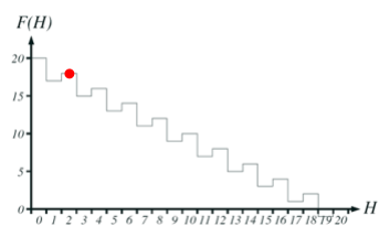
these situations?
-
There’s two methods:
-
Adaptive walks from a peak
-
By measuring how long it takes to walk to the peak of a
hill, we can figure some things out.
-
For example, if the adaptive walk length is really small, is likely to be really high.
-
Or, if it’s greater than , it’s likely to be a long path problem.
-
Fitness distance correlation
-
Plotting fitness against Hamming distance in scatter plots
can help visualise the shape of the fitness landscape:
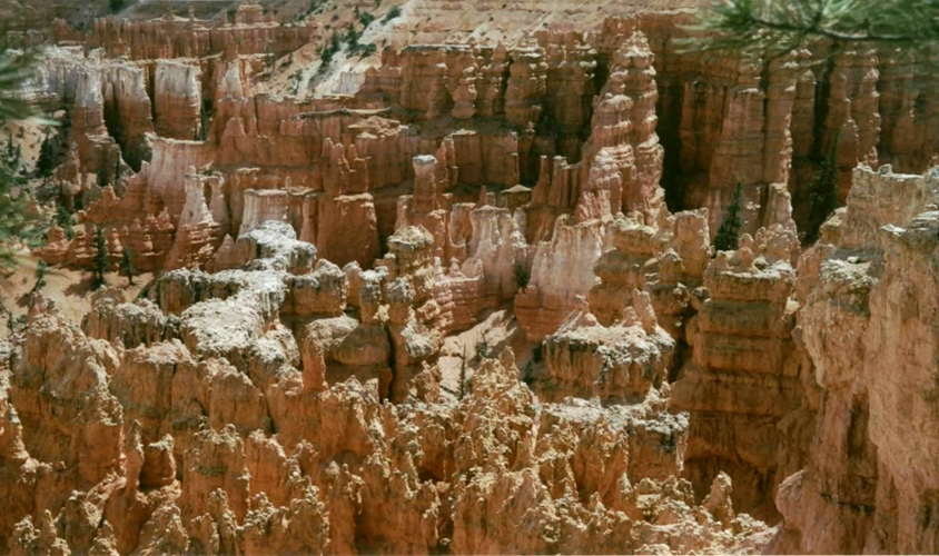
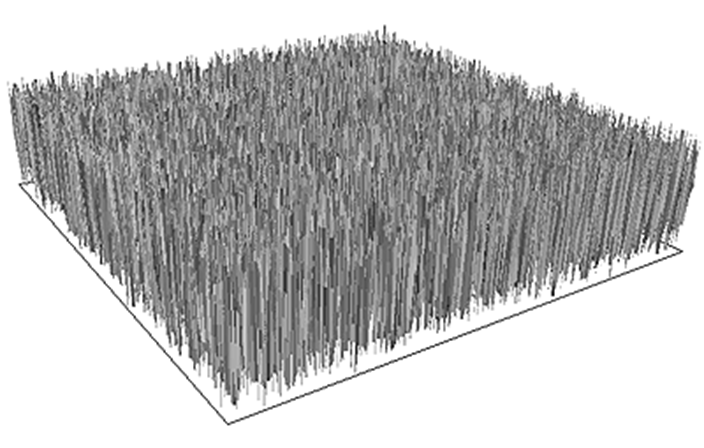
Examples: Biological Landscapes
-
A biological example of a fitness landscape would be beak
size:
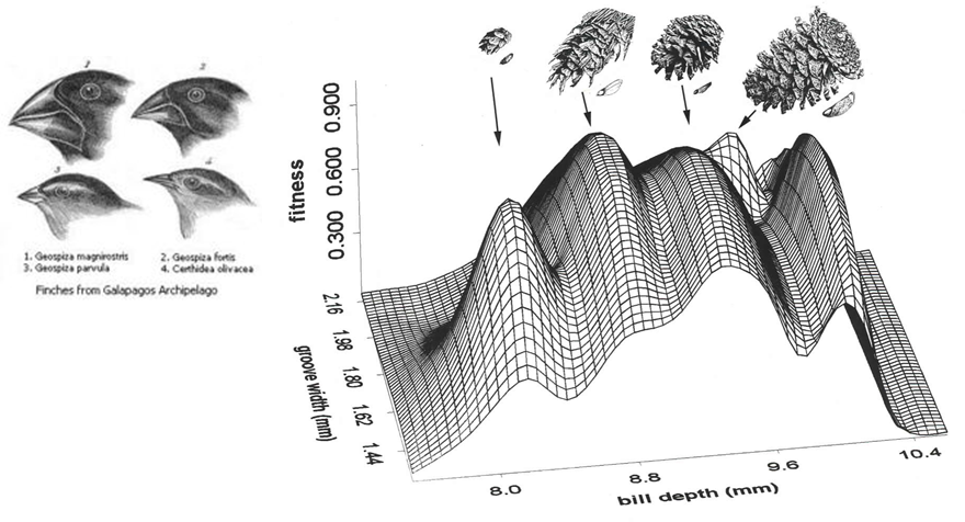
-
Different beak sizes match different seeds, hence why there
are multiple peaks.
-
This graph is in trait space, which means the axis are traits of the individual, such
as bill depth.
-
But, if we think about this for a second, we realise things
aren’t quite so simple.
-
What actually affects these “fitness”
values?
-
There’s a whole sequence of things that derive fitness for individuals:
-
Nucleotide sequences (ACTGGGGACAC)
-
→ Amino acid sequence
-
→ Protein shape
-
→ Protein function
-
→ Trait value
-
→ Fitness contribution
-
That’s a lot of steps!
-
Evolution only really affects the nucleotide sequences, so
those are the things we should be graphing.
-
But that’s so complex, that we’ll be spending
the rest of our lives drawing one graph!
-
Plus, that fitness contribution is still epistatically
dependent on other proteins.
-
So, what? We cry and switch modules?
-
Not today! We create small windows on real
landscapes.
Complications
-
When we’re trying to reason with real-life evolution,
we can’t map out an entire fitness landscape.
-
Instead, we “peek” and look at small windows of
the real landscape.
- How?
-
There are different ways to do this.
-
One way is looking at populations of different gene
mutations:
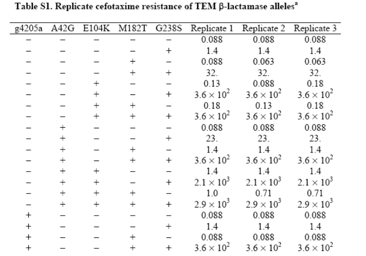
-
... and then constructing accessible evolutionary paths
from that data:
-
Another way is a series of one-step peeks into a
high-dimensional space.
-
So, instead of mapping the whole landscape, we map points
with a radius (like a flashlight in a horror game):

-
We can even use protein folding.
-
These long protein strings ultimately determine
fitness.
-
We can “fold” these proteins, and each protein
folds in a different way.
-
They can fold well, or they can fold... not so well.
-
If the protein folds the way it should, that means that
protein has a low fold energy, and if it doesn’t fold
the way it’s supposed to, that protein has a high fold
energy.
-
We can map this fold energy to fitness.
-
We want proteins that fold properly, so a low fold energy
is high fitness, and a high fold energy is low
fitness.
-
It gets even more complicated...
-
There’s the whole Wright vs Fisher and the relevance
of epistasis.
- Things like:
-
Spaces and operators
-
Individuals vs Populations
-
Sexual populations vs Asexual populations
-
Noise and dynamic landscapes
- Coevolution
-
Designing landscapes
-
“If we’re on a hill anyway, we’re always
going to go uphill.”
-
“Other peaks and optima do not matter.”
-
“So epistasis doesn’t matter,
either.”
-
“Dumbass.”
-
“Epistasis and local optima are a big deal for
natural populations.”
-
“They’re biologically significant too,
dickhead.”

Fisher and Wright, hard at work.
-
How do populations go from one peak to another?
-
To do that, we need to partially ignore the local fitness
gradients.
-
This can happen in small populations (or multi-dimensional populations).
-
We can represent populations in a certain way.
-
We can represent it as a point in an allele frequency space, which refers to the set of all possible vectors that
denote the frequency of alleles in each loci of the
gene.
-
Movements due to selection in sexual populations move to
adjacent points in this space... sometimes.
-
Doesn’t make sense? Not a problem, here’s an
example:
|
Example
|
|
|
0
|
0
|
0
|
1
|
1
|
1
|
1
|
|
0
|
0
|
0
|
1
|
1
|
1
|
1
|
|
1
|
0
|
0
|
1
|
0
|
0
|
0
|
|
1
|
1
|
0
|
0
|
0
|
1
|
1
|
|
2
|
1
|
0
|
3
|
2
|
3
|
3
|
-
The blue rows are the genes, and are bit
strings.
-
At each column, the value in red is the sum
of the 1 values in blue.
-
So the first column is ‘2’
because there are 2 1’s in the column
above.
-
The red row is our allele frequency
vector.
-
It is our representation of this
 population in our allele frequency
space. population in our allele frequency
space.
|
-
You know, all this time we’ve been assuming that
distance = genetic differences (Hamming distance).
-
Like, the genotype AAB has a distance of 1 away from
ABB.
-
But what if that’s not strictly true?
-
For example, could you get from:
-
in just one step?
-
With mutation, no.
-
With crossover...?
-
000000000000000000 +
-
111111111111111111 =
-
000000000111111111
-
So, we can get from that genome to that other genome in one
move!
-
If that’s so, then they should have a distance of 1,
right?
-
That means they should be neighbouring, right?
-
Terry Jones, back in 1995 when he was writing his PhD,
would say “yes”.
-
Richard would say “no”, though.
-
So as you can see, the representation of a genome is very
important.
-
It determines what movements are natural and what fitness
landscapes exist.
-
When you design EAs, you need to choose your encoding
wisely.
Sex
-
Just quickly, let’s go over the two-fold cost of sex, or the cost of males.
-
Let’s say individuals can produce 4 eggs per
generation.
-
Asexuals can produce 1 → 4 → 16 → 64 eggs in
4 generations
-
With sexuals, it’s halved, because half of
individuals are males who can’t produce eggs.
-
So sexuals can produce 1 → 2 → 4 → 8 in 4
generations. Far less!
-
In summary, males contribute genes but they don’t
increase egg production or population growth.
-
So, why do we have males?
-
It’s a bit more complicated than just maths.
-
Males also provide parental investment.
-
Plus, egg production in females might be increased to
compensate, so egg production is the same after all.
-
But why do humans sexually populate at all? Why don’t
we asexually reproduce?
-
Let’s find that out...
-
There’s two ways to make new individuals with
sex:
- Reproduction
-
Recombination
-
With reproduction, each parent has two diploids.
-
Their sex cells takes one of the two strands, called
haploids.
-
When they “have sex”, a haploid from
‘daddy’ and a haploid from ‘mummy’
join together to form a diploid again: a new
individual.
-
We’re not really making any new genes; we’re
shuffling them around.
-
With recombination, we make new genes for the children.
-
There’s two kinds of recombination:
-
Chromosomal reassortment: Chromosomes are split and shuffled in hard-coded cutoff
points that are the same every time
-
Crossover: Chromosomes are split and shuffled in randomly selected
cutoff points
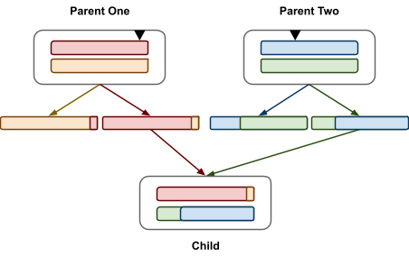
Linkage Equilibrium
-
When you have crossover, the chance that two genes are
still together after recombination depends on their physical linkage.
-
Physical Linkage: the tendency for alleles to travel together during
recombination due to physical proximity on the
chromosome.
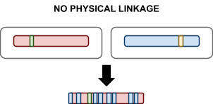
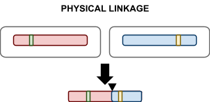
-
In uniform recombination there is no physical linkage, because all genes are
chosen at random.
-
In one-point crossover, there is physical linkage, because adjacent genes on one
side of the cutoff point remain together.
-
When you do recombination, you can either join
alleles:
-
How do the frequencies of these combinations change?
-
Linkage Equilibrium: joint frequencies of alleles are product of marginal
frequencies
-
In other words, we say that there is no over (or under)
representation of combinations of alleles.
-
Using maths, it means f(AB) = f(A) * f(B)
-
f(A) means the frequency of ‘A’ genes in the
chromosomes
-
Linkage Disequilibrium is the deviation of the observed frequency of gene pairings
from the expected frequency.
-
Basically, it’s any deviation from linkage
equilibrium.
-
What does that really mean?
-
Let me use an example from Wikipedia.
|
Example: Two-loci and two-alleles
|
-
Let’s say you have a chromosome with
two loci (positions) and two possible
alleles for each loci:
ab
aB
Ab
AB
-
Let’s say the frequencies of getting
each of these are:
|
Haplotype
|
Frequency
|
|
ab
|

|
|
aB
|

|
|
Ab
|

|
|
AB
|

|
-
Those are the frequencies of the haplotypes
(frequency of the combination of alleles
together).
-
Here’s the frequencies of the alleles
individually:
-
If the loci and alleles are independent of
each other, then you could say that:
-
In other words, the frequency of gene
‘ab’ is just the frequency where
the first loci picks ‘a’ and the
second loci picks ‘b’.
-
That’s linkage equilibrium.
-
However, linkage disequilibrium is where
the loci and alleles are not independent of
each other, and observed frequencies like don’t follow this
pattern.
|
-
Remember physical linkage?
-
Uniform crossover has no physical linkage because random
loci are picked for the child.
-
That means there’s no way for two joint alleles to be
over or under represented, because they have an equal chance
of being selected or not selected.
-
So uniform crossover is really good at returning alleles to
linkage equilibrium.
-
However, what about one-point crossover?
-
If the joint alleles are close together, they’ll have
high physical linkage, so they’ll be over
represented.
-
If the joint alleles are far apart, they’ll have low
physical linkage, so they’ll be closer to linkage
equilibrium.
-
How do we get out of physical disequilibrium?
-
Have sex! (use sexual recombination, I mean)
-
A benefit of sexual recombination is that it reduces
linkage disequilibrium.
-
Under-represented combinations are created more than
they’re destroyed.
-
Over-represented combinations are destroyed more than
they’re created.
-
Why do organisms have sex? Why can’t they just
asexually mutate for everything?
-
What’s so good about reducing linkage
disequilibrium?
Fisher / Muller Hypothesis
-
Let’s take our two-loci two-allele example
again.
-
Let’s say we have a big population of them.
-
Upper-case alleles are more beneficial than lower-case
ones.
-
However, through mutation, individuals can only go
from:
-
This is linkage disequilibrium: the frequency of AB does
not correlate with the frequency of A and B individually
because mutation can’t get to AB.
-
With an asexual population, we get:
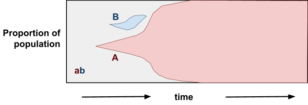
-
Individuals mutate and get Ab and aB, but since they
can’t mutate to be both, there’s
competition.
-
Eventually, Ab wins, and the beneficial B allele dies
out.
-
However, with a sexual population:
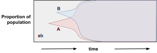
-
With crossover, we don’t need mutation to reach AB;
an Ab could mate with an aB and get an AB!
-
This removes competition between the two segregating
alleles.
-
In other words, sex is advantageous because it allows
alleles to be selected for independently.
-
Let’s look at this with bit-strings.
-
Let’s say you have two initial genotypes:
|
00100000000010000001 (3)
|
00000100000010001000 (3)
|
-
With asexuals, you can only produce more of these two
genotypes.
-
Yeah, there’s mutation, but that’s quite
slow.
-
But sexuals can produce all of these:
|
00100000000010000001 (3)
|
00100000000010000000 (2)
|
|
00100000000010001001 (4)
|
00100000000010001000 (3)
|
|
00100100000010000001 (4)
|
00100100000010000000 (3)
|
|
00100100000010001001 (5)
|
00100100000010001000 (4)
|
|
00000000000010000001 (2)
|
00000000000010000000 (1)
|
|
00000000000010001001 (3)
|
00000000000010001000 (2)
|
|
00000100000010000001 (3)
|
00000100000010000000 (2)
|
|
00000100000010001001 (3)
|
00000100000010001000 (3)
|
-
Way more variation!
-
Variation is good, because it means we can explore the
search space better.
Muller’s Ratchet
-
Muller’s Ratchet is like the opposite of the Fisher /
Muller hypothesis.
-
Instead of good alleles coming together, this is about
removing bad alleles.
-
Let’s say you have a population of good
genotypes.
-
That means almost any mutation would make the individual
worse than better.
-
Like in the “methinks it is like a weasel”
where you have a sentence that’s only one character
off from being perfect.
-
With asexuals, mutations that bring the fitness down cannot
be recovered (at least not easily). That’s like a ‘click’ of the ratchet
you can’t go back on.
-
But with sexuals, you can cross two half-unmutated
individuals to recover the original unmutated
individual.
-
Populations are finite
- No elitism
-
No back mutations
-
No beneficial mutations (mostly because all genotypes are
good)
-
This is cool because deleterious mutations are more common
than beneficial ones.
-
However, this only applies to finite populations, and
according to Charlesworth, the time for a ratchet click is
very long in large populations.
|
|
💡 NOTE
|
|
|
|
Richard skipped over the deterministic mutation
hypothesis, so I won’t go over it in the
notes.
Let’s hope it doesn’t come up in
the exams!
|
|
-
Ok sex is cool and all but what about from a computing
point of view?
-
Is using sex any better than a simple hill-climber or
something?
-
The examples I used before had no local optima, so a
hill-climber would make all our problems go away, plus
it’d be easier to implement.
-
In the next section, we’ll go over why sex is good
for computer scientists too.
Crossover in EAs
Focussing Variation
-
Let’s have a look at uniform crossover again.
-
Let’s say we’re uniform crossover-ing these two
bit-strings:
|
0
|
0
|
1
|
1
|
0
|
1
|
0
|
1
|
|
0
|
1
|
1
|
1
|
0
|
0
|
1
|
1
|
-
Have a look at the first bit. It’s always going to be
zero, won’t it?
-
No matter which bit-string uniform crossover picks, that
bit will always be zero.
-
All bits where the two individuals agree on the same bit
won’t change:
|
0
|
0
|
1
|
1
|
0
|
1
|
0
|
1
|
|
0
|
1
|
1
|
1
|
0
|
0
|
1
|
1
|
|
-
|
?
|
-
|
-
|
-
|
?
|
?
|
-
|
-
What uniform crossover is effectively doing is just
mutation on those bits where the individuals are different (where I’ve put the green question marks).
-
This concept is called focussing variation, or ‘focussing search’.

I know it’s hard to, but you must focus!
-
Let’s have a look at the Hurdles problem.
-
The X axis is the number of zeroes.
-
The Y axis is the fitness.
-
You’ll notice that there’s dips when the number
of zeroes is odd, and peaks when it’s even.
-
Let’s say we have an individual on a peak. How do we
get to the next highest peak?
-
For example, let’s say, we have 18 ones and 2
zeroes.
|
11111011111101111111
|
|
-
Let
 be the length of the bit-string.
-
How would asexuals (mutation) vs sexuals (uniform
crossover) fare with this problem?
|
Asexuals
|
Sexuals
|
|
Let’s say each bit has a  chance of being mutated. chance of being mutated.
We have two zeroes we need to mutate to get to
the next peak.
However, we can’t just mutate one of the
two zeroes, because we’d fall into the
dip, get worse fitness, and this individual will
die out.
We must mutate both zeroes at the same
time.
The chance of that is  , or , or  . .
To generalise that, the chance of mutation
getting to the next peak is  , where is how big the hurdle is. , where is how big the hurdle is.
|
Let’s say there’s two individuals
at the two zeroes peak:
11111111111101101111
11011011111111111111
Remember, uniform crossover is the same as
mutation on the bits that are different:
11111111111101101111
11011011111111111111
--?--?------?--?----
If we were to do mutation on those differing
bits, we’d need 4 successive ones to get
to the next peak.
The chance of that is  . .
To generalise that, the chance of uniform
crossover getting to the next peak is  , where is how big the hurdle is. , where is how big the hurdle is.
|
-
Sexuals are way more likely to solve the problem quicker
than asexuals!
-
The chance a sexual solves the problem does not depend on
the length of the bit string, but asexuals do.
-
In other words, sexuals are way better at
“jumping”, or performing better in fitness
landscapes with gaps.
-
Can hill-climbers do that? Pfft... no.
-
Let’s compare one point crossover with uniform
crossover.
-
We have two bit-strings:
|
0
|
0
|
1
|
0
|
0
|
0
|
0
|
0
|
0
|
0
|
0
|
0
|
1
|
0
|
0
|
0
|
0
|
0
|
0
|
1
|
|
0
|
0
|
0
|
0
|
0
|
1
|
0
|
0
|
0
|
0
|
0
|
0
|
1
|
0
|
0
|
0
|
1
|
0
|
0
|
0
|
|
-
|
-
|
?
|
-
|
-
|
?
|
-
|
-
|
-
|
-
|
-
|
-
|
-
|
-
|
-
|
-
|
?
|
-
|
-
|
?
|
-
With uniform crossover, you can make up to 16 different
bit-strings from these two.
-
With one-point crossover, you can make 3 unique
bit-strings.
-
That sounds like crap, but hear me out.
-
The chance of getting each bit-string in one-point
crossover is
 (on average; assuming all differing genes are
equidistant).
(on average; assuming all differing genes are
equidistant).
-
Let’s say that both uniform crossover and one-point
crossover gives you the children you want.
-
Which one are you gonna pick:
-
The one with exponential complexity or
-
The one with polynomial complexity
-
You’re going to pick the polynomial one, right?
-
If one-point crossover is going to give you the children
you want anyway, you might as well use that and get the
individuals you want faster than with uniform crossover or
mutation.
-
Yeah, uniform crossover gives more variation, but
it’s variation you don’t need. The group of
resulting individuals will be ‘diluted’ with
useless individuals of low fitness.
-
What’s the difference between:
-
the individuals you’d get from one-point crossover
and
-
the individuals you’d get from uniform
crossover?
-
Differing bits that are close together are unlikely to be
recombined.
-
Here’s an example:
|
0
|
0
|
0
|
0
|
0
|
0
|
0
|
0
|
0
|
1
|
0
|
0
|
0
|
0
|
0
|
0
|
0
|
0
|
0
|
0
|
|
0
|
0
|
0
|
0
|
0
|
0
|
0
|
0
|
0
|
0
|
1
|
0
|
0
|
0
|
0
|
0
|
0
|
0
|
0
|
0
|
|
-
|
-
|
-
|
-
|
-
|
-
|
-
|
-
|
-
|
?
|
?
|
-
|
-
|
-
|
-
|
-
|
-
|
-
|
-
|
-
|
-
With one-point crossover, what’s the chance of
getting a child with two ones?
-
It’d be very low, because the cutoff point would have
to hit that sweet spot to get the one from the red parent
and the one from the blue parent.
-
What about now?
|
0
|
1
|
0
|
0
|
0
|
0
|
0
|
0
|
0
|
0
|
0
|
0
|
0
|
0
|
0
|
0
|
0
|
0
|
0
|
0
|
|
0
|
0
|
0
|
0
|
0
|
0
|
0
|
0
|
0
|
0
|
0
|
0
|
0
|
0
|
0
|
0
|
0
|
0
|
1
|
0
|
|
-
|
?
|
-
|
-
|
-
|
-
|
-
|
-
|
-
|
-
|
-
|
-
|
-
|
-
|
-
|
-
|
-
|
-
|
?
|
-
|
-
Now there’s a huge chance that the bits are
recombined, because there’s a much bigger window for
the cutoff point.
-
In fact, it’s unlikely that they won’t get
recombined.
-
In summary, two close differing bits are unlikely to both change because of their physical linkage.
-
This is the bias of one-point crossover.
-
What if we could use this, though...?
-
What if the bits we want to keep the same are kept close
together?
Schemata and Building Blocks
Schemata Theorem
-
A schema is a general representation of a set of individuals that
share common bits.
-
For example, given this set of bit-strings:
|
1
|
1
|
0
|
1
|
0
|
1
|
0
|
0
|
0
|
0
|
1
|
0
|
0
|
1
|
0
|
0
|
0
|
0
|
|
0
|
1
|
0
|
1
|
0
|
1
|
0
|
0
|
0
|
0
|
1
|
0
|
1
|
0
|
1
|
0
|
0
|
1
|
|
1
|
1
|
0
|
1
|
0
|
1
|
0
|
0
|
1
|
0
|
1
|
0
|
0
|
1
|
0
|
0
|
1
|
1
|
|
1
|
1
|
0
|
1
|
0
|
1
|
0
|
0
|
1
|
1
|
0
|
1
|
0
|
1
|
1
|
0
|
1
|
1
|
|
*
|
1
|
0
|
1
|
0
|
1
|
0
|
0
|
*
|
*
|
*
|
*
|
*
|
*
|
*
|
0
|
*
|
*
|
-
If you’re sick of these coloured tables already,
it’s this:
-
The genes that are the same for individuals in the schema
are represented as ‘0’ or ‘1’.
-
The genes that can be anything for individuals in the
schema are represented as ‘*’.
-
The order of a schema is how many specific genes there are in the
schema.
-
For example, **1**0*1* has an order of 3.
-
The defining length is the distance from the first specified gene to the last
specified gene.
-
For example, **101** has a shorter defining length than 1***0.
-
You can also say “shorter order” if you have a
small defining length.
-
The schema fitness is the average fitness of all genotypes that fit that
schema.
Building Block Hypothesis
-
Holland (1975), Goldberg (1989) and others said that
schemas are the reason why GAs work so well.
-
They say that:
-
GAs find small schemas
-
Crossovers put small schemas together to make bigger
ones
-
It keeps making bigger schemas until the whole problem is
solved
-
These are Building Blocks: low-order, short defining length schema of above average
fitness, that can be put together with crossover to make
bigger building blocks.
-
Mitchell and Forrest set out to test this.
-
They created an idealised problem with a special kind of
building block.
-
You’ve seen it before: the Royal Road!
|
Bit string
|
Fitness
|
|
1111 0000 0000 0000
|
8
|
|
0000 1111 0000 0000
|
8
|
|
0000 0000 1111 0000
|
8
|
|
0000 0000 0000 1111
|
8
|
|
1111 1111 0000 0000
|
16
|
|
0000 0000 1111 1111
|
16
|
|
1111 0000 1111 1111
|
24
|
|
1111 1111 1111 1111
|
32
|
-
As you can see, if you
had:
-
1111 0000 0000 0000 (8) and
-
0000 0000 1111 1111 (16)
-
You can put these two building blocks together with
crossover to form:
-
Mitchell and Forrest did this, but it’s still nothing
a hill-climber can’t do.
-
In fact, a hill-climber does this better than a GA!
-
Plus, it’s a simpler algorithm!
-
How embarrassing...
-
So what can GA do better than hill-climber?
-
Well, that whole ‘sexuals being good at
jumping’ thing from earlier was pretty good.
-
That’s from Shapiro and Prugel-Bennet (1997)’s
‘two wells’/’basin with a barrier’,
and Thomas Jansen (2001)’s
‘Gap’/’jump’ function.
-
Also, Watson himself made a hierarchical modular
building-block problem (called H-IFF) where hill-climber can solve it in
 , whereas GA with tight linkage can solve it in
  .
.

-
That’s great and all, but so what?
-
Who cares? Do YOU care?
-
GAs can solve some things better than hill-climbers,
but...
-
... it’s not a standard GA, or even a
‘standard’ problem.
-
We’re just solving problems we’ve invented
ourselves.
-
We’re not solving any practical engineering problem,
and it has nothing to do with biology.
-
Can we show that GAs are the best thing ever in a more
simple model?
Two-Module Model
-
We’re going a bit biological in this one.
-
Nucleotide sites within a gene are grouped both
functionally and physically by virtue of shared
transcription and translation.
-
In other words, this is a simple form of biologically-real
modularity.
|
|
|
gene 1 (determines how strong you are)
|
|
|
|
|
gene 2 (determines how smart you are)
|
|
|
|
|
|
1
|
1
|
0
|
1
|
0
|
0
|
|
|
|
|
1
|
1
|
1
|
1
|
1
|
1
|
|
|
-
Obviously, we want to be strong and smart 😎 so we’d want to maximise the
ones in both these genes.
-
Let’s say that mutations in the same gene have
stronger synergy than mutations in different genes.
-
In other words, fitness increases exponentially with each
good mutation; the closer we are to a perfect gene, the more
important the mutations are.
-
You wanna see the fitness functions of this?
|
Fitness Function
|
Description
|
|
|
This fitness function only takes into account
gene 1.
As you increase the number of beneficial
mutations in gene 1, the fitness of the whole
thing exponentially increases.
|
|
|
This fitness function takes into account gene 1
and gene 2.
As you increase the number of beneficial
mutations in gene 1 and gene 2, the fitness of the whole thing
exponentially increases.
Notice there’s a spike where gene 1 and
gene 2 are perfected. That’s our global
optima! We want our individuals to reach
it.
The problem here is that a hill-climber can
solve this really easily. It can just go up the
slope of gene 1 or gene 2, and then slide along
the edge of the landscape towards the global
optimum.
What’s Richard gonna do about that?
|
|
|
He added noise!
This isn’t a fitness function, but
whatever. This is the noise he added.
More specifically, it’s random epistasis
among all loci.
It was generated with random fitnesses between
0.5 and 1.
|
|
|
This is what the fitness function looks after
overlaying (by multiplying) the noise.
Now, on the ridge of the fitness landscape,
there are many small peaks, or local sub-optima.
Hill-climbers are going to get stuck in
there.
|
-
So, who’s going to win this one?
-
The hill-climbers?
-
Or the genetic algorithms?
|
Hill-Climbers
|
Genetic Algorithms
|
|
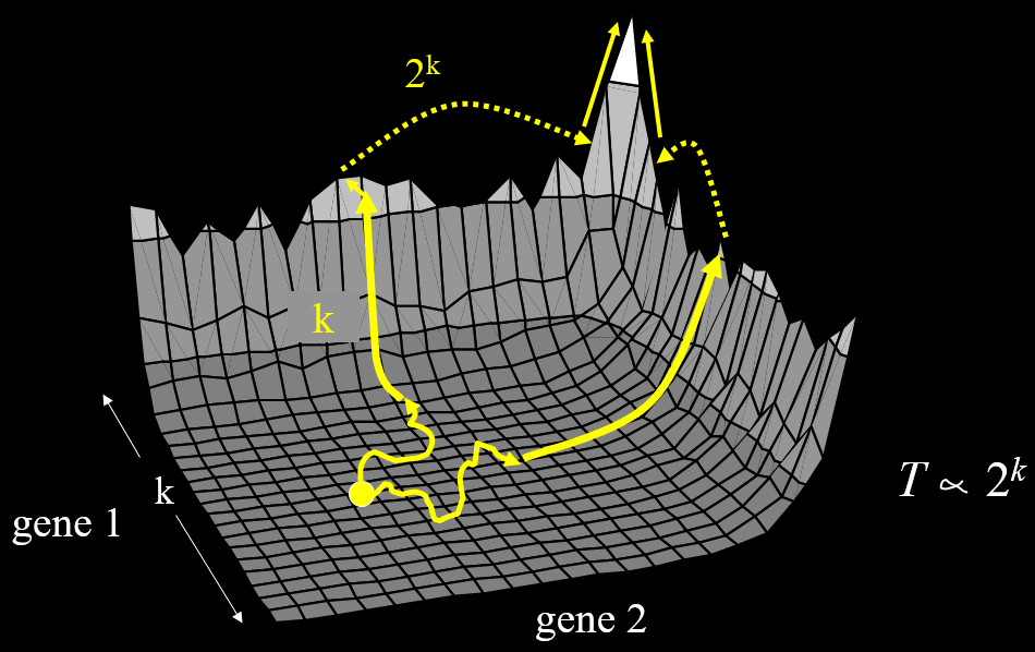
A hill-climber can easily find the peak of one
gene.
The problem is finding the peak of the other
gene without disrupting the first one.
Given the genes are loci long, it’ll take a
hill-climber steps to get to one peak.
The hill-climber will have to mutate just the
right genes to ‘jump’ to the highest
peak.
It’ll take  steps to do that. steps to do that.
Therefore, hill-climbers can solve this in
exponential time.
|
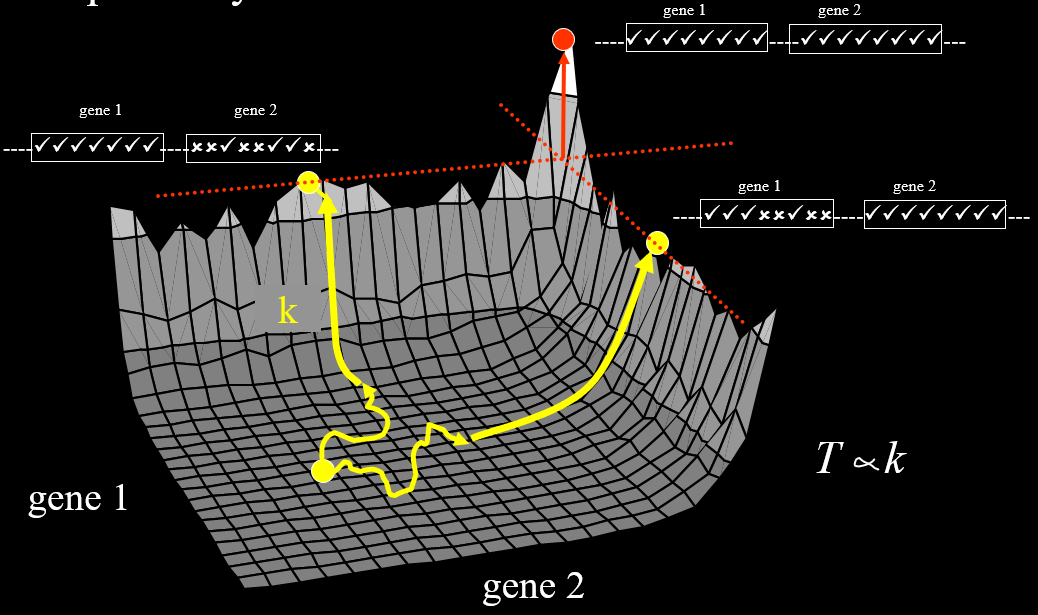
Like hill-climbers, GAs can find the peak of
one of the genes easily.
It takes steps to reach one of the peaks.
However, once two individuals reach the peaks
of the other two genes, they can crossover and
make a child at the global peak. This only takes
one (lucky) step!
Therefore, GAs can solve this in polynomial
time.
|
-
Hill-climbers reach the individual gene peaks, but
couldn’t find the global optimum, even after 1000
generations.
-
GAs with uniform crossover are similar: they struggle to
find the global optimum.
-
GAs with one-point crossover find the global optimum at
generation 58.
Richard’s 3000-page report PDF on the two-module
model
-
In conclusion: if you want to be strong and smart, use
one-point crossover.
-
Mutations on genes finds good building blocks
-
Recombination on building blocks finds good genotypes
-
Mutation on individual nucleotides finds good genes
-
Recombination on genes finds good genotypes
Coevolution
-
There are two definitions of coevolution:
“Evolution as a result of biological
interactions”
“An evolutionary change in a trait of the individuals in
one population in response to a trait of the individuals in a
second population, followed by an evolutionary response by the
second population to the change in the first”
-
The main thing to take away from this is reciprocity.
-
Hence, coevolution can also be called reciprocal evolution.
-
What’s the difference between normal and reciprocal
evolution?
|
Normal evolution
|
Coevolution
|
|
With normal evolution, the agent of selection
does not change as a result of the evolutionary
response it causes.
In other words, individuals are always selected
based on the same criteria, no matter what has
happened.
|
With coevolution, the agent of selection does
change as a result of the evolutionary response
it causes.
In other words, individuals are selected based
on the situation and what’s happened so
far in the algorithm.
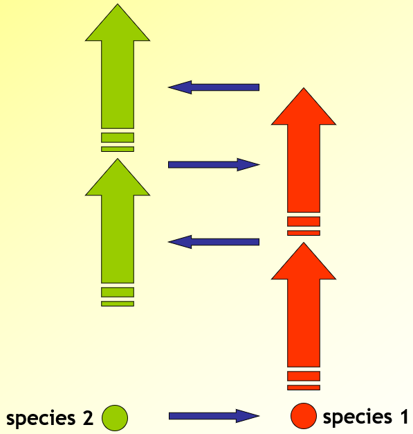
^ Positive feedback mechanism
|
-
In layman’s terms, with coevolution, you have two (or maybe more) populations that engage in “arms races”
to improve and increase in fitness together.
-
Think of it this way:
-
When you catch a cold, it sucks. But it doesn’t last
forever; eventually, you recover from it. Your body
remembers that strain of cold so you won’t catch it
again.
-
However, some of the cold viruses in your body survived;
these survivors will go on to be the next generation of
stronger cold viruses, that’ll one day come back
around and infect you again.
-
This cycle continues, and forms the basis of competitive
coevolution.
Missed opportunity for a covid joke? Maybe.
Pairwise vs Diffuse
-
In pairwise coevolution, we just have two homogenous populations that try to
one-up each other. Similar to the common cold example from
before.
-
Here’s the example from the slides:

-
We have antelopes and a field of grass.
-
The antelopes eat the grass. Oof.
-
The grass doesn’t like being eaten, so it evolves to
be tougher.
-
The antelopes have a harder time eating it, so they evolve
harder teeth.
-
This pairwise arms race continues on.
-
In diffuse coevolution, we have multiple populations on both sides, and one
population could affect any of the other populations,
directly or indirectly.
-
Here’s an adaptation of the example from the
slides:
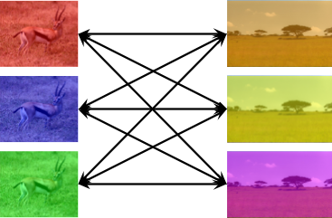
-
We have red, blue, and green antelopes, as well as orange,
yellow, and magenta grass.
-
A case of diffuse coevolution could be:
-
Let’s say the red antelopes eat the orange grass.
-
The orange grass starts to evolve a poison that makes the red antelopes sick.
-
The red antelopes stop eating the orange grass and start eating the yellow and magenta grass, and some of them evolve stronger stomachs.
-
However, a blue antelope has tasted the orange grass and finds it delicious. The poison for the red antelopes is a taste enhancer for the blue antelopes!
-
Now, all the blue antelopes stop eating the other grasses and only eat orange grass.
-
The orange grass evolving poison has affected:
-
Red antelopes: they start eating other grass / evolve stronger
stomachs
-
Blue antelopes: they only eat orange grass now. New diet could affect
them in other ways
-
Yellow and magenta grass: they are no longer being eaten by blue antelopes, but they are being eaten by red antelopes, so the pressure to evolve defence mechanism will
change to suit red antelopes
Sasaki & Godfray Model
-
Let’s say we have two populations: parasites and
hosts.
-
The hosts have a resistance to parasites.
-
The parasites have a virulence (counter-resistance) to
hosts.
-
However, resistance and virulence is negatively
proportional to fitness.
-
So hosts and parasites need to “spend” some of
their fitness to increase resistance / virulence.
-
They enter a cycle, where:
-
Hosts increase in resistance so parasites won’t
infect them
-
Parasites increase in virulence so they can infect
hosts
-
They both reach a point where they can’t increase
resistance and virulence any longer
-
Hosts give up increasing resistance, because it
doesn’t matter either way anymore: virulence is so
high that high resistance and low resistance doesn’t
matter, so we might as well have low resistance so we get
our fitness back.
-
Parasites give up increasing virulence for the same reason:
they don’t need so much virulence anymore, so they get
fitness back.
-
The cycle continues again.
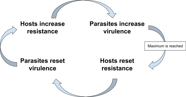
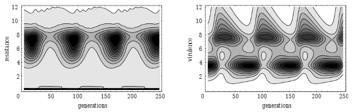
Heat maps when resistance and virulence have low fitness
cost
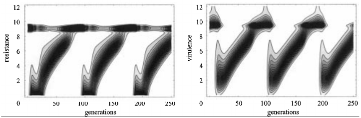
Heat maps when resistance and virulence have high fitness
cost
Coevolution in GAs
-
In a normal GA, you have a population of individuals and a
fitness function that takes one individual.
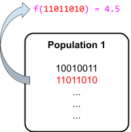
-
In coevolution, you have two populations, and two fitness
functions that return the fitness of an individual given the
other individual in the other population.
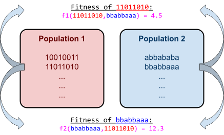
-
Can you answer this question: how good are you at
chess?
-
It’s hard, right? It depends.
-
How about this question: how good are you at chess compared
to a grandmaster?
-
What about this: how good are you at chess compared to a
complete novice?
-
This is subjective (internal) fitness: how good an individual is compared to a sample of
individuals in the other population.
-
There’s also objective (external) fitness, which is the raw fitness of an individual, but this
isn’t needed for coevolution; it’s mostly an
analysis thing.
Have you heard of Watson’s Gambit? It’s where
you
make a coevolutionary algorithm play for you.
-
There are different kinds of fitness evaluations:
-
Controllers: e.g. pursuer / evader
-
Instances / classifiers: e.g. lists / sorters
-
Symbol production and understanding: e.g.
communication
-
Two player games: chess, drafts, backgammon
-
More complicated games, like poker
-
To calculate subjective fitness for an individual, they
need to play against opponents.
-
Who should they play against?
-
Everyone? That’s expensive...
-
One opponent? The results will be noisy and
inaccurate...
-
A sample? Now you’re talking!
-
So, you’ve co-evolved a population and now
they’re all kick-ass chess players.
-
But is there really one best individual who can beat
everyone?
-
What if you had one individual who was good at winning by
being aggressive...
-
... and another individual who was good at winning by
planning ahead?
-
Surely, different individuals will only do well against
different opponents.
-
If the population represents a diverse set of strategies,
how should scores against many players be combined?
🤔
-
... what? You’re asking me?
-
I don’t know. I just write the notes.
Why use Coevolution
-
There’s several reasons why:
-
Implicit fitness function
-
You don’t have to explicitly define a fitness
function.
-
For example, you don’t have to define what makes a good chess
player.
-
Each population defines the problem for the other, and the
fitness is determined by the rules of the game.
-
Gradient engineering - arms race
-
Even if you did have a fitness function, how would you know
if it provided an appropriate gradient?
-
In other words, even if you did define what makes a good
chess player, how would you know if individuals would be
able to evolve and climb their way to being a
grandmaster?
-
With coevolution, the populations gradually increase in
difficulty automatically.
-
Even if you did have a fitness function and it had a good
gradient, would it be open ended?
-
In other words, when an individual maxes out your fitness
function, are they really the best they could possibly be at
chess? Or is there still room for improvement?
-
Because coevolution doesn’t define a strict fitness
function, the populations are free to explore the limits of
the game itself.
-
The results may surprise you!
-
There’s more examples of coevolution:
-
Input list creator vs list sorter
-
Cellular automata classifiers vs initial conditions
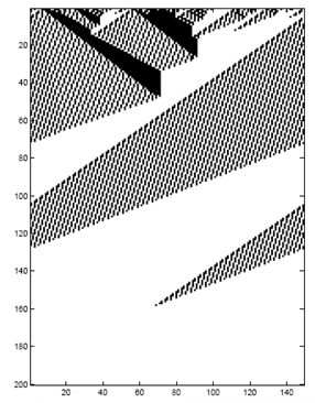
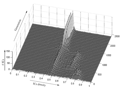
-
Coevolution has so much freedom that, sometimes, it might
not evolve what you want it to evolve.
-
What do you actually want?
-
A player that beats every possible strategy?
-
A player that would rather win and lose than draw all the
time?
-
A player that gets the best average score against all
players?
-
A player that writes the notes for you? (I wish...)
Problems with Coevolution
-
It’s not the best thing in the world, though.
-
There are problems with it:
-
Disengagement / loss of gradient
-
This is where one population beats all individuals of the
other population, so nobody ever improves.
-
Imagine playing against a grandmaster chess player.
-
Assuming you’re not a grandmaster also, you’re
not gonna learn anything because you’ll just get your
arse handed to you.
-
The grandmaster won’t learn anything either because
it’ll be easy for them.
-
This is where a population’s strategies are too
specific to the opponents they’re playing.
-
If you do machine learning, this is very similar to
overfitting.
-
Imagine you play against a player who always plays
aggressively.
-
The only strategy you’ll learn is how to hammer
someone who plays too aggressively.
-
So when you play against a different opponent, your
strategy won’t work so well, and you’ll be
crap.
-
This is where populations follow a cycle of
strategies.
-
Think rock paper scissors:
-
Rock → Scissors
-
Scissors → Paper
-
Paper → Rock
-
If pop1 all plays rock, pop2 will all play scissors.
-
Now that pop2 all plays scissors, pop1 will all play
paper.
-
Now that pop1 all play paper, pop2 will all play
rock.
-
This cycle will continue forever and no populations will
actually reach a good optimum.
-
This is where populations collude to be mediocre
together.
-
If both populations get the same scores whether they try
hard or not, why should they try hard?
-
Both populations will just play mediocre and get the same
scores.
-
These are called mediocre stable states.
Cooperative Coevolution
-
I wanna talk about bumblebees.
-
Aren’t they cool? They go into flowers and collect
nectar, and create honey.
Me busting my ass writing these notes
-
The system with the whole flowers producing nectar to
entice bees while also spreading pollen is a pretty cool
thing.
-
Almost too cool...
-
How did they get like that?
-
Did bees and flowers hold a meeting to decide on a
mechanism that benefits them both?
-
No! Bees and flowers evolved like this through cooperative coevolution!
What is Cooperative Coevolution
-
Cooperative coevolution is where individuals from a number of populations
collectively solve some problem together.
-
So, rather than chess players, hosts / parasites, pursuers
/ evaders etc., we have multiple agents working on
different parts of the same problem.
-
With competitive coevolution, the fitness function returns
the fitness of the individual in the context of an opponent
individual.
-
With cooperative coevolution, we have a “shared domain model” and we often have more than two populations.
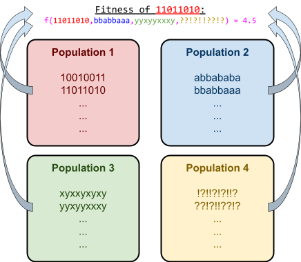
-
When we find the fitness of an individual, we pick the best
individuals of every other group to calculate it with.
-
However, the main difference is how we interpret the whole
thing.
Competitive vs Cooperative
-
In competitive coevolution:
-
The solution to the problem is an individual from one of
the populations
-
In cooperative coevolution:
-
The solution to the problem is a collection of individuals,
one from each population
-
However, the individuals don’t know the
difference!
-
It’s not like we tell them “ok you gotta
cooperate with these lot”
-
Individuals perform exactly the same whether it’s
competitive or cooperative.
-
The only thing that’s different is how you interpret
the results: get a solution from one individual, or a
group.
-
In both cases, individuals’ fitnesses are sensitive
to the genetics of the other populations.
-
Competition only exists within populations.
-
When you think about it, opponent individuals simply
“set the scene” or “change the criteria of
success” for their competition.
-
In other words, population 2 is just the (dynamic) environment population 1 evolves with respect
to.
|
Example: Opponents “setting the
scene”
|
-
Let’s say we have two
populations.
-
We want to find the fitness of an
individual in population 1, named
 . .
-
We sample one opponent to calculate this
with (crap, I know, but whatever), and we select the opponent
 . .
-
So we can calculate fitness like
this:

-
Easy, right?
-
Well, let’s change the way we look at
it.
-
What if we made a new function:

-
You could say that, in this very instant,
the individuals in population 1 are evolving
with respect to the fitness function
 . .
-
Our opponent, , simply plays a part in defining the
fitness function of population 1.
-
Do you see how opponents “change the
criteria of success” for their
competition?
|
-
In summary, the mechanics behind competitive and
cooperative coevolution is the same.
-
The only difference is how you interpret the results.
-
Here’s an example:
-
Let’s say you’re doing coevolution against two
badminton players.
-
What do you want out of this algorithm?
-
The best badminton player for singles?
-
Then it’s competitive; pick an individual from either
population.
-
This is adversarial coevolution.
-
The best badminton pair for doubles?
-
Then it’s cooperative; pick the best individuals from
both populations.
-
This is compositional coevolution.
Badminton yeeaaaaa 🏸🏸🏸
Divide and Conquer
-
Competitive coevolution is about gradient
engineering.
-
Ensuring that populations are as good as each other, so
they can improve on one another.
-
However, cooperative coevolution is different.
-
Cooperative coevolution is about problem
decomposition.
-
We want each population to focus on a subproblem.
-
Their fitness is represented by how well each
individual’s sub-solutions come together to
collectively solve the whole problem.
-
Sound familiar? This is the divide and conquer approach in
general computer science!
-
Divide and conquer is used everywhere, including:
-
Designing cars 🚗
-
Designing space shuttles 🚀
-
Designing processors 💻
-
Managing businesses 💼
-
Town planning
-
Algorithm design (especially modular ones)
-
You can even apply this to optimisation, if it’s
modular enough:
-
Train schedule timetabling for each city
independently
-
Postal routes
-
Optimising a design by optimising sub-systems
-
Is there a case where divide and conquer doesn’t
work?
-
Yeah: consider the prisoner’s dilemma. It’s a classic example of how optimisations of
subproblems does not always constitute the optimisation of
the whole problem.
-
If we evolve prisoners independently, they’ll both
evolve to betray each other.
-
However, if we evolve pairs of prisoners (basically modelling a pair of prisoners as a single
individual), they’ll evolve to ally.
If you’ve done Intelligent Agents and are doing Game
Theory,
you’re probably sick of prisoner’s dilemma by
now.
-
So, divide and conquer will only work if individual
optimisations of each part provide optimisation of the
whole.
-
But how do we actually split up a problem? That’s the
real question.
-
We’ll go into more detail next topic, in Modularity!
-
When you think about it, cooperative coevolution is very
much like building blocks and crossover:
-
Problems are decomposed into subproblems
-
Subproblems are put together to solve the bigger
problem
-
There’s a big difference though:
-
Building block sub-problems are independent, whereas in
cooperative coevolution, they might not be independent (sub-problems might only make sense in the context of the
bigger problem).
-
There might be no way of evaluating a sub-solution on its
own.
Modularity
Types of modularity
-
There are two kinds of modularity:
-
Repetition
-
Where parts of the evolved structure have repeated
modules
-
Fingers on a hand
-
Components on a circuit board
-
Cells of a multicellular organism
Remember this?
-
Functional decoupling
-
Where different modules have different roles in the bigger
system.
- Examples:
-
Nervous system and digestive system
-
Peripherals for a computer
-
Procedures in software code
-
Proteins
-
Modularity implies re-use.
-
Repetition→ re-use in a single device / organism
-
Functional decoupling → re-use in other devices /
variants
-
Either way, there is self-contained functionality.
-
Modularity reflects the inherent structure of the problem
space.
-
Repetition implies self-similarity in sub-problems.
-
For example, say you had the problem of driving 10 cars to
Southampton.
-
You could split this problem up with repetition: the
problem of driving 1 car to Southampton, but 10 times.
-
Functional decoupling does not imply this.
-
Identifying modular subnetworks in bigger, complex networks
is useful for understanding how it all works (network dynamics).
-
It may look like this:
Modular subnetworks in a complex network
-
This is an example of structural representation: with connections between
modules.
-
In evolving complex systems, we can identify modules based
on how much they affect other parts of the system.
- For example:
-
If we modified one bit of the system and there was no
interference to this other bit, they’re probably in
different subsystems.
-
If we modified one bit and there was loads of interference
in this other bit, they’re probably in the same
subsystems.
-
This is an example of functional representation: with changes affecting modules.
Concepts of modularity
-
There’s two ways to view modularity:
-
Structural (topological / connectedness)
-
This refers to the number of connections within a module
(intramodular), or between modules (intermodular)
-
Functional (dynamics, behaviour, fitness)
-
This refers to how changes in one module affects results of
other modules, in terms of dynamics, behaviour, fitness
etc.
-
Keep in mind that structural is not the same as
functional.
-
They are implicitly related, though.
-
When you think of modularity, you may think that modules
barely affect each other at all.
-
But that’s not necessarily true.
-
Sure, there are more intramodular dependencies (connections inside the module itself) than intermodular dependencies (connections between modules), but that doesn’t mean they’re not
important.
|
Your nervous system and digestive system are
two different subsystems of your body.
What would happen if you used your nervous
system to stop your breathing and die?
Your digestive system would shut down,
too.
After all, you can’t eat anything if
you’re dead.
|
And no: let’s assume zombies don’t
exist.
|
-
If that’s too weird of an example of modules
critically affecting each other, try this:
|

UNLIMITED POWER
|
In a tower PC, the power supply
‘supplies’ power to the components
through sleeved cables.
You could say the ‘power system’ is
separate from other ‘modules’, like
the motherboard or the RAM.
But what if your power supply fails? Nothing
would be able to run anymore.
In that sense, the power system still
critically affects other systems.
|
-
Modularity is when intramodular dependencies have a greater
effect on fitness than intermodular dependencies,
right?
-
How can inter-connections be critical, yet systems exhibit
meaningful modularity?
-
Isn’t that high coupling?
-
It’s complicated...
Examples
Simon’s “nearly-decomposable” systems
-
A “nearly-decomposable” system is a system with two properties:
-
“the short-run behaviour of each of the component
subsystems is approximately independent of the short-run
behaviour of the other components”
-
“in the long run the behaviour of any one of the
components depends in only an aggregate way on the behaviour
of the other components”
-
Uhh... ok? What does that mean?
-
It means that:
-
In the short run, components are pretty much independent of
each other.
-
In the long run, however, the behaviour of components
depends on the aggregate of the other components.
-
Some examples will help clear this up.
-
Here’s two examples that Richard came up with in the
lecture:
|
The moon revolves around the Earth, and Saturn
exists also, with their 82 moons.
In the short run, the moon revolves with little
to no impact from Saturn and their moons, and
vice versa with Saturn’s moons.
In the long run, they still do affect each
other. Perhaps, after 100 years, our moon is
shifted a couple metres from its orbit because
of the gravity from Saturn and its moons (calculated by taking Saturn’s, and its
moons’, mass as an aggregate).
|
|
|
|
In the short run, people from the UK do not
affect what people from the US think and do (unless they’re explicitly talking to
them).
In the long run, however, the collective
opinions and actions of people from the UK do
affect what people in the US think and do, and
vice versa for them.
Maybe.
|
-
If you don’t like those examples, here’s some
that Simon came up with:
|
The Combination Lock
|
|
Let’s say you had a combination lock with
10 dials, and each having 100 positions (so a lot more advanced than the picture on the
left).
To unlock it, you need to start with the first
lock, guess the right number for that lock, and
sequentially go through and guess each lock
until you’ve got them all.
You always hear a ‘click’ whenever
you get one lock right.
The problem here is that modules are completely independent of each other.
|
|
|
The Watchmaker’s Parable
|
|
|
We have a watchmaker, Mr. Casio, who creates
watches by putting together 1000 components
sequentially.
If Mr. Casio is interrupted, he has to start
from scratch.
Richard, on the other hand, puts together 10
components, made out of 10 sub-components, made
out of 10 modules.
If Richard is interrupted, he can just start
again on the latest module / sub-component /
whatever he was working on.
Richard has intermediate stable modules, but
Mr. Casio does not, meaning he builds watches
more efficiently.
We have modules and hierarchy, but the problem
here is that making modules is just a
deterministic sequence of steps.
You can’t create a fitness function for
this, so there’s no way to show the
functional representation of modules.
|
|
Heat Exchange
|
|
We have a building with many rooms and many
cubicles.
Cubicles start at different temperatures, and
heat travels between them.
Heat exchange rate is greater for cubicles in
the same room than in different rooms.
In the short run, a cubicle’s temperature
is only affected by other cubicles’
temperatures in the same room.
In the long run, cubicles can also be affected
by the average temperatures of cubicles in the
other rooms: the heat travels from those rooms
to our room.
It’s a hierarchical modular dynamic
system, which is nice, but the problem here is
that there’s no real problem to solve. It
has nothing to do with evolvability.
|
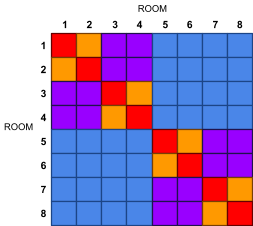
Heat exchange coefficients of cubicles in
rooms
|
-
Picky picky... there’s always a problem, isn’t
there?
-
We want to show GAs with crossover perform better than GAs
without crossover using an example with modularity.
-
These examples aren’t the answer, but we can draw
some inspiration.
Modularity in EC
-
Do you remember NK landscapes?
-
It’s a fitness landscape with two variables:
-
- number of variables
-
- number of dependencies between variables
-
It has inter-dependencies, but no modularity.
|
NK landscapes
|
Royal Roads
|
NKC (clustered)
|
|
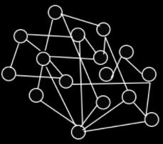
|
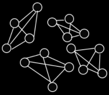
|
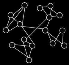
|
|
Inter-dependencies between loci
No modularity or hierarchy
|
Inter-dependencies in building blocks
Building blocks are the modules
No hierarchy
|
Inter-dependencies between modules
There are lower level and higher level
modules
Most benefit comes from optimising lowest level
modules
|
-
You wanna see some more examples of modularity in synthetic
landscapes?
-
The intra-block column represents the fitness function of one
individual module.
-
The inter-block column represents the fitness function of the whole
landscape with each successive complete module.
|
Name
|
Intra-block
|
Inter-block
|
Resultant landscape
|
|
Royal Roads
|

|

|
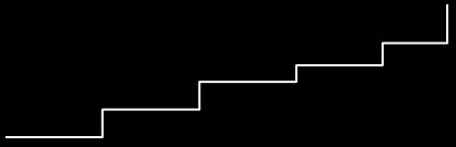
|
|
Concatenated Traps
|

|

|
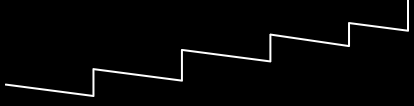
|
|
NKCs
|
|
|
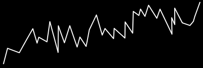
|
|
Hierarchical IFF
|
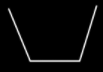
|
|
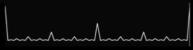
|
-
In royal roads, a module only affects the fitness until it’s all
complete, which is why the intra-block landscape spikes
right at the end.
-
As you complete modules, the fitness increases linearly,
which is why the inter-block landscape is just a linear
function.
-
In concatenated traps, a module has a dip, but goes back up right at the end,
hence the name ‘trap’.
-
As you complete the modules, like the royal roads, the
fitness increases linearly.
-
In NKCs, it’s a bit hard to discern because the epistasis is
random, but the fitness still increases in proportion to the
completed modules.
-
In Hierarchical IFF, a module is complete when it has all ones or all zeroes,
but not a mixture.
-
The fitness of the overall landscape depends on how you
complete the modules. We’ll see this in more detail in
a sec, but the point is, it’s not linear like the
others.
Hierarchical IFF as a Dynamic Landscape
-
Let’s go into more detail in this Hierarchical IFF (HIFF) function.
-
Let’s say we have two genes, and they can either be 0
or 1.
-
If they’re both 1, we get more fitness!
-
If they’re both 0, we get more fitness!
-
If they’re different, then we don’t get as much
fitness.
-
Here’s the fitness function of HIFF:
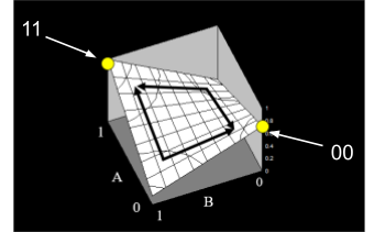
-
If that’s hard to visualise, here’s the same
function flipped on its side:
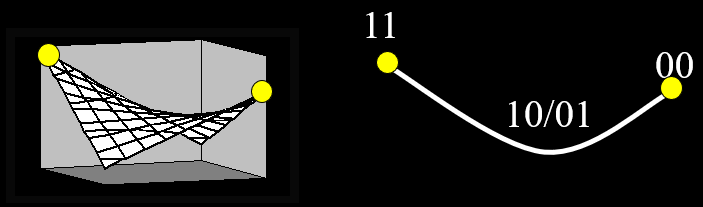
-
The two peaks are where both genes are 11 or 00, and the
dip is where they’re different (01 or 10).
-
We’ll visualise it like this:
|
Pairwise inter-dependency
|
|
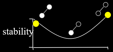
|
-
Using this as a base, we’ll make a landscape
with:
-
Intra-dependencies that are more important than the
inter-dependencies (modularity)
-
Inter-dependencies that are still important
-
In a way you can actually understand?!
-
You may think it’s crazy, but read on; things are
about to start making sense.
-
Next, we’re going to increase the complexity of this
landscape a bit.
|
Uniform inter-dependency
|
|
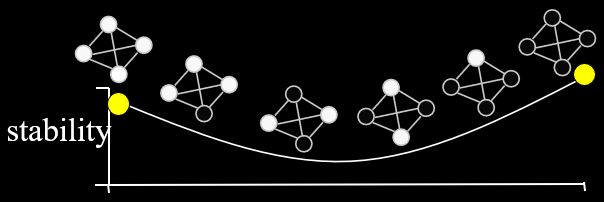
|
-
We’ve added two more genes, and all genes are
dependent on each other.
-
However, it’s still not modular.
-
Then how about we add some modules?
|
Modular inter-dependency
(4 genes, 2-storey hierarchy)
|
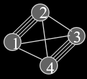
|
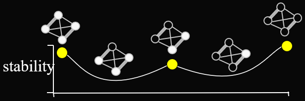
|
-
Now, 1-2 and 3-4 are modules!
-
They have strong intra-dependencies, and weaker (but still
prevalent) inter-dependencies.
|
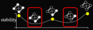
If you have incomplete modules, you will be
down in a dip.
|

If you have complete modules, but the
modules’ aggregate (all 1’s or all
0’s) don’t match, you’ll get a
local optimum.
|
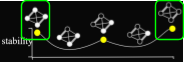
If you’ve completed all modules and all
module aggregates agree, you’ll get the
global optimum.
|
-
That’s pretty cool! Now we have:
-
Intra-dependencies matter more than inter-dependencies (modules: complete modules is better than incomplete
ones)
-
Inter-dependencies are still important (getting all modules correct is better than getting a few
correct)
-
We can go even further, and add more genes and larger
modules:
|
Modular inter-dependency
(8 genes, 2-storey hierarchy)
|
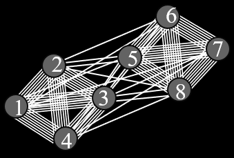
|
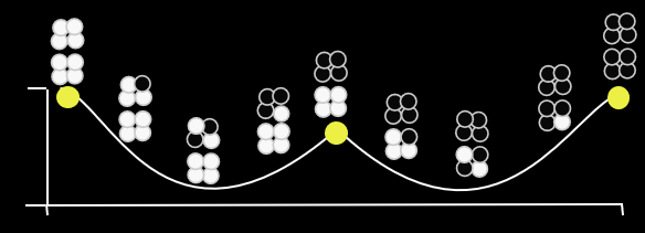
|
-
It’s pretty much the same as before, but with more
genes, larger modules and wider fitness saddles.
-
In general, things are more
“fine-grained”.
-
We have enough space to add another hierarchy, by creating
another sub-module in our existing modules:
|
Modular inter-dependency
(8 genes, 3-storey hierarchy)
|
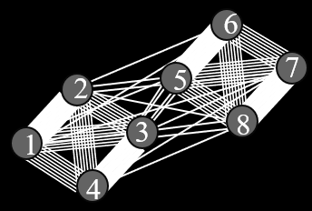
|
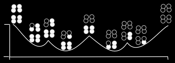
|
-
Here, we’ve got more local optima!
-
So, what’s so good about HIFF? We already have
modularity and stuff in the royal roads.
-
The difference is that hill-climbers can solve royal roads,
but not HIFF.
-
Hill-climbers can climb up the steps of the fitness
landscape pretty easily.
-
However, hill-climbers have to flip a lot of bits to get
from one optimum to the next.
-
Look at the fitness landscape in the 8-gene 3-storey
example above.
-
If you’re on the local optimum a quarter from the
left/right (with a half-complete module and a complete module), you’d have to flip 2 bits to get to the next local
optimum (middle).
-
From the middle, you’d have to flip 4 bits to get to
the global optimum (sides).
-
With HIFF, the number of bits you need to flip doubles each
optimum. No way a hill-climber is going to do that!
|
|
💡 NOTE
|
|
|
|
Of course, if you’re on a quarter local
optimum, you can flip two bits to get to the
global maximum.
However, HIFFs are meant to have way more
dimensions (or ‘storeys’) than just
these three. Have a look at the HIFF landscape
just above where I compared it to royal roads, concatenated trap, and NKC!
|
|
-
There’s many different ways of representing this
clustered dependency network:
|
Name that I’ve given it
|
Image
|
|
Really Messy Graph
Similar to the diagrams above, it’s just
all the genes represented as nodes, and the
dependencies represented as edges.
|
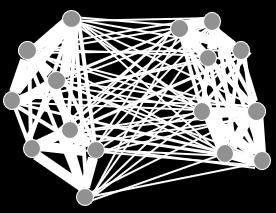
|
|
Plum Pudding
(no relation to the J. J. Thompson model)
Genes are represented as nodes again, but
sub-modules are circle-grouped genes and modules
are circle-grouped sub-modules and so on.
|
|
|
Hierarchical Chocolate Chip Cookie (HCCC) Network
A more hierarchical representation. The bottom
graphs are just Really Messy Graphs for each
submodule, then the next levels up show the
inter-dependencies.
|
|
|
Tree
It’s just a hierarchical tree showing the
structure of the modules and their
dependencies.
|
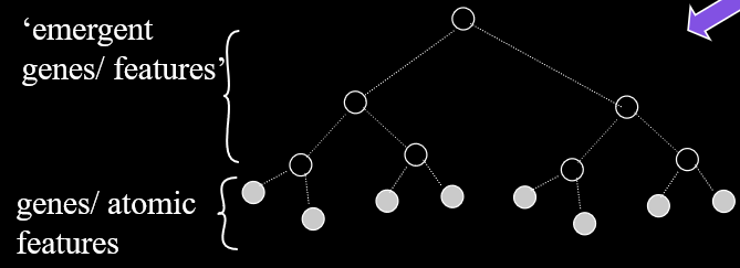
|
-
There’s other ways to represent this too, that
demonstrate aggregate effects better:
|
Normal Graph
|
Aggregate Graph
|
Squiggly Tree
|
Normal Tree
|
|
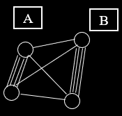
|
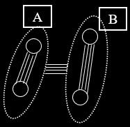
|
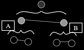
|
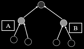
|
|
Modular system of four variables (like
above).
|
Instead of uniformly connecting every node to
each other, we abstract a whole module with an
oval and the dependencies to-and-from it are
based on aggregate states.
|
Instead of using ovals, aggregate states are
represented as different shades of nodes.
Higher tree levels represent higher levels of
abstraction, in other words,
‘phenotypic’.
|
The same as Squiggly Tree, but with edges
instead of squiggly brackets.
|
-
In summary, modulation is epic.
-
It appears everywhere through nature, and helps simplify
bigger problems.
-
It also gives us an example where GAs with crossover
triumph over hill-climbers.
-
However, building block genes need to be next to each other
for GA with crossover to work.
-
We’ve been looking at building blocks that look
like:
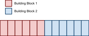
-
But what if it looks like:

-
They’re still modules! Their loci just aren’t
adjacent.
-
Crossover wouldn’t be able to help us here.
-
The difference here is the representation.
-
Oh my! Would you look at the name of the next
section!
Representations
-
Before, we’ve been representing individuals as
strings:
-
Bit strings: 0101101010
-
Normal strings: Methinksiusdfhdsf7w4ruinjkfvbh
-
Letters as genes: ACTGACACACGTAGCTAC
-
This isn’t what biology does, though.
- In biology:
-
DNA is transcribed into amino acids
-
Amino acids fold into proteins
-
Proteins control cell division and differentiation,
creating a variety of cells
-
The cells form together to make a creature
-
The creature exhibits phenotypes which determine
fitness

-
In our algorithms, we have a direct function from genotypes
to fitness.
-
In real life, genotypes (DNA) determine the phenotype (eye colour, arm length etc.), which determines fitness.
-
The mapping from genotypes → phenotypes is pretty
complicated. It depends on:
-
Epistasis: effect of a mutation depends on genetic background (other genes)
-
Pleiotropy: one gene influences many traits
-
Redundancy: many genotypes map to a particular phenotype
-
Neutrality: some mutations on some backgrounds have no fitness
effect
-
This all affects the evolvability of a species.
-
Those are the properties that affect the mapping, but what
are the properties of the mapping that affects the
evolvability?
-
Connectivity (or selective accessibility): functionally similar beetles should have very similar
genetics
-
Bias: good phenotypes are evolved to have a bias in the mapping (beetles with horns are biased over beetles with wings on
their ankles)
-
Modularity - Functional Decomposition: genes that affect function of the heart should be mostly
independent of genes that affect function of the ears
-
Modularity - Repetition: mutations in genes that affect your fingernails will
probably affect your toenails too (nails are repeated modules)
Graphs (TSP)
-
In the graph colouring problem, we can represent a possible solution with a string.
-
We number the nodes from
 to
to  , and in our string, the
  th position is the colour of the th node.

-
Easy game, easy life!
-
We can even use mutation and crossover on this.
-
Thing is, it won’t make for a very good solving
algorithm.
-
However, mutation and crossover won’t work:
-


 (invalid: permutation has node 2 twice)
-
 ,
,
-

 (invalid: permutation has node 2 twice)
-

 (invalid: permutation has node 3 twice)
-
So what are we going to do? 😭 Switch modules?
-
No! Don’t give up yet, we got this!
-
Our problem lies in our representation.
-
Remember, GAs are heuristic search mechanisms that work by
exploring points on a search space with a similar cost to
the previous points.
-
To do this, our variation operators (mutation and crossover) need to produce alterations that change cost as
little as possible.
-
In TSP, it’s not the nodes that incur a cost:
it’s the edges.
-
Instead of representing nodes, we can represent the edges
instead.
-
Then, we can build operators that preserve as many edges as
possible.
-
To do crossover with edges, we can use edge recombination.
-
We take some edges from parent 1
-
We take some edges from parent 2 that don’t clash
with our existing choices
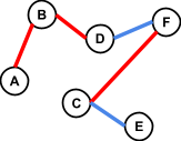
-
We fill in the gaps to make it a legal tour again
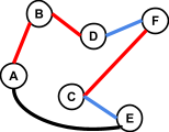
-
To do mutation with edges, we use the algorithm called 2-Opt.
-
Split the path into three partitions
CD DE EF FA AB BC

-
Reverse the middle partition
CD AF FE ED AB BC
-
We’re almost done; time for the actual mutation!
Tweak the ‘neighbours’ of the second partition
in the first and third partitions so that they enter and
leave the reversed partition.
CA AF FE ED DB BC
-
Boom! You’ve mutated the path.
-
However, sometimes 2-opt isn’t enough.
-
In those cases, you can use 3-opt, which is similar but with more partitions.
-
It’s more powerful, but also more disruptive.
-
You can use this to perform a fast neighbourhood search,
actually.
-
It’s fast because you don’t have to recompute
the cost of paths with 2-opt and 3-opt; you can derive the
new cost based on what edges you’ve changed.
Structured Representations
-
Before, we were representing paths and solutions.
-
How could we represent structure, like a graph?
-
We could use matrices!
-
With artificial neural networks, we could have a matrix of weights.
-
We can go from matrices to strings by putting each row next
to each other:

-
Since we can use normal mutation and crossover on strings,
we can use the same operations on matrices.
Variable-size Parameter Sets
-
One problem is variable-size parameter sets.
-
In other words, what if we don’t want our matrix to
be fixed?
-
What if we want it to be of a variable size?
-
If we tried to crossover a 10x10 with a 15x15, it’s
not clear what to do.
-
We can fix this with relative connections!
-
Instead of explicitly saying
-
“node 1 is connected to node 3 with weight
4”
-
“node 1 is connected to the node 2 spaces along, with
weight 4”.
-
Where “the node 2 spaces along” means
“node 1 + 2”, which is “node
3”.
|
node 1
|
node 2
|
node 3
|
|
+2, 0.3
|
+3, -2.0
|
-1, 1.2
|
-2, 0.4
|
-
Now, when you do crossover with two graphs, it
doesn’t matter how many nodes there were.
Trees
-
When we represent trees, we need to define a mutation and
crossover operation.
-
For an example, let’s look at abstract syntax trees.
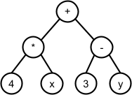
(4 * x) + (3 - y)
-
When you evolve these, that’s called Genetic Programming (GP).
-
One possible problem that can be solved with GP is system identification: finding an equation that describes a system.
-
When you mutate a tree, you can change a leaf or a binary
node:
|
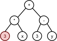
(3 * x) + (3 - y)
|
(4 * x) * (3 - y)
|
-
When you do crossover, you exchange subtrees:
-
This is cool and all, but variation can be quite
disruptive.
(29 * x + 33) - (5 + x)
→
(29 * x + 33)(5 + x)
-
However, in binary trees, most nodes are leaves, so
it’s not so bad.
-
Sometimes, subtrees won’t contribute to the
formulae.
-
Like subtrees that are multiplied by zero:
-
Through evolution, these subtrees will grow and bloat the tree.
-
It’s not all bad though: when you have bloat, it
reduces the disruptiveness of the mutation.
-
Sometimes, a bit of bloat is an advantage to balance out
the disruptiveness of mutation.
-
Of course, bloat has two downsides:
-
Reduces interpretability of the formulae (it gets confusing)
-
Produces over-complicated formulae (leads to overfitting)
-
You can reduce bloat by incurring a fitness cost when trees
get too big.
Grammar Based Representations
-
Do you remember context-free grammars?
-
If not, go refresh yourself on them in the ToC notes.
-
Here, they’re called L-systems.
-
They look like this:
-
However, that’s not useful for evolution.
-
What would be useful for evolution would be something like
this:
-
Body → Arm Arm
-
Arm → Hand
-
Hand → Finger Finger Finger Finger Thumb
- ...
-
How do we represent these?
Cellular Encoding
-
One way is encoding a grammar in a tree, known as cellular encoding.
-
This is a way to represent artificial neural nets with a
grammar.
-
How do we get from a tree to a grammar?
-
This is a special tree that modifies a neural net with just
one internal node.
-
Uh... huh? Trees that modify neural nets?
-
We have a grammar for our trees:
-
Command → PAR | SEQ | END | ...
-
SEQ → Command Command
-
PAR → Command Command
- ...
-
Then, we evolve instantiations of this grammar as
trees.
-
We use these trees to generate ANNs.
-
I’ll show you:
|
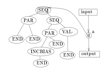
|
So here, we have one cell in the neural net,
and it’s pointing to the root of our
tree.
The root node has the command SEQ, and that
command will be applied to our cell here.
SEQ means divide the cell sequentially in two, and make those two cells point to
the children.
|
|
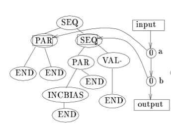
|
Now, our ‘a’ cell was split into
two, ‘a’ and ‘b’, and
they point to the root node’s children,
PAR and SEQ.
Let’s perform the PAR command on that
‘a’ cell.
PAR means divide the cell in parallel and make the children cells point to the
children nodes.
|
|

|
‘a’ was split into ‘a’
and ‘c’ in parallel, meaning they
both come from the input instead of before where
b’ came after ‘a’.
This keeps on going until the neural net is
fully generated.
|
-
This exhibits properties of repeated modularity and
self-similarity, which can be exploited for tasks that have
said self-similarity.
-
For example, if we were evolving a frog with four legs, you
could use the “PAR” node twice to split a node
representing a leg into four nodes representing four
legs.
-
Or something.
Turtle Graphics
-
Do you remember the Logo programming language?
-
Basically, there’s a cursor on the screen, and you
can use commands to move the cursor around to draw
stuff.
-
It’s pretty cool, but it’s only used for
drawing stuff.
-
You can create grammars to draw stuff in Logo:
-
S → Forward 10, Right 1, S
-
→ Forward 10, Right 1, Forward 10, Right 1, S
-
→ Forward 10, Right 1, Forward 10, Right 1, Forward
10, Right 1, S
- ...
-
This grammar keeps drawing forward and going right
slightly, to make a circle:

-
You can do branching too:
-
Forward 10, [Right 10, Forward 20], Left 10, Forward
20
-
You can make even more complex grammars and make actual
trees:
Advanced Representations
-
Remember how we represented graphs?
-
What if those graphs were, like, lifelike mechanisms?
-
And the edges could expand, like rods?
-
So the mechanisms could move?
-
You can make fish!
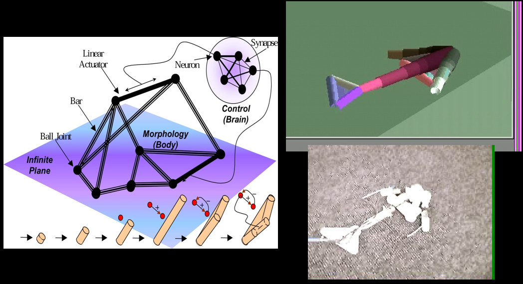
-
Then evolve those fish and make land creatures!
-
Then evolve those land creatures and make dinosaurs!
-
Then evolve those dinosaurs and make apes!
-
Then evolve those apes and make humans!
-
Do you like automata?
-
I like automata.
-
How about an automata that can make a tree? (Structure-defining tree-based FSMs)
-
Or a ribcage (I know, it’s a bug with six legs)?
-
Or even you...?
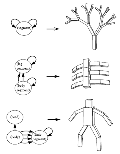
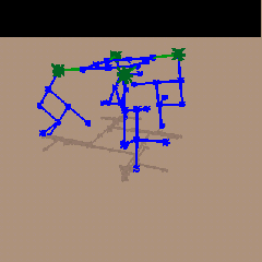
-
We can represent ANNs with grammars, but how do we actually
evolve them?
-
There’s this algorithm called NEAT (NeuroEvolution of Augmented Topologies), and this guy used it to play Pac-Man!
-
In short, NEAT is a genetic algorithm for evolving neural
nets.
-
Instead of evolving just the neural net’s weights, it
also evolves the structure, with the nodes and
everything.
Artificial Life
-
Do you watch Futurama?
-
Have you seen the episode “A Clockwork
Origin”?
-
In it, nanobots are put on a lifeless planet, and they
evolve into greater and greater robotic creatures.
-
That’s an example of artificial life.
-
There’s many different kinds of artificial life, as
we’ll see...
Concept, Motivation, Definitions
-
What actually is artificial life?
“Artificial Life is a field of study devoted to
understanding life by attempting to abstract the fundamental
dynamical principles underlying biological phenomena, and
recreating these dynamics in other physical media - such as
computers - making them accessible to new kinds of experimental
manipulation and testing.”
-
TL;DR, it means representing the abstract principles of
life, and recreating them (usually in a computer) so we can manipulate and test it.
-
Life on earth: “life as we know it”
-
Artificial life: “life as it could be”
-
Why do you survive? Why does anything survive?
-
It depends on how good they are at:
- Finding food
-
Avoiding predators
-
Finding mates (for sexuals)
-
Among other things, like:
-
Metabolic functions
-
Lifecycle functions
-
However, there’s nothing hard-coded into us that says “if you’re good at finding food, you’re
allowed to pass on your genes”.
-
In our algorithms, we hard-code this, with things like “if you have the most ones in your bit-string,
you’re selected for reproduction”.
-
The difference is:
-
Implicit fitness / selection: an individual that produces many offspring, in the
context of its environment, is fit.
-
In real life, there are no set rules or fitness functions;
the organisms that manage to reproduce are the ones that
carry on their genes.
-
Explicit fitness / selection: an individual that performs well at a task/problem has
‘high fitness’ and is permitted to
reproduce.
-
In simulations, if you’re bad at the given task, you
will not reproduce.
-
There are two ways of thinking about artificial life:
-
Strong artificial life: It doesn’t matter if it’s biological or
mechanical; if they both exhibit the same dynamical
properties, they’re both living.
-
Weak artificial life: Mechanical life doesn’t have the same complexity
and isn’t made of the right stuff; it’s not
living.
-
There’s two categories of artificial life:
-
Dry artificial life: artificial life made mechanically, like computer
simulations, robots etc.
-
Wet artificial life: artificial life made with biological components and
‘wet stuff’
-
There’s different approaches to wet artificial
life:
-
Minimal genome: take a real bacteria, remove all unnecessary genetic
material with trial and error until you get a super minimal
bacteria
-
Artificial genome: synthesise a minimal metabolic system based on logical
design (create your own custom genome of a bacteria, take an
existing bacteria and replace its DNA with your custom
genome).
-
Self-organisation in biomolecules: get a flask of biological ‘goo’, shake it
around, and let it ‘self-organise’ and emerge
spontaneously (people think this doesn’t work because there’s
too much entropy, there’s not enough
compartments)
-
Synthetic DNA: synthesise DNA and put it into an artificial cell
That’s not what I meant by ‘wet artificial
life’...
Examples
-
Have people actually made artificial life before?
-
Of course they have! Let’s look at a few.
Karl Sims Creatures
-
Karl Sims made box creatures in a physical world with
sensors and actuators.
-
He trained them to do different things, like swim around,
move around, chase laser pointers etc.
-
I’ve already shown you this video before, but whatever.
-
Sims used an explicit fitness function, for things like how
far they could move, how close they moved to the laser
pointer etc.
He even made, um... sperm?
Framsticks
-
Framsticks is a freeware artificial life simulator.
-
It’s more modern than Karl Sims, and you can download it and use it yourself!
-
However, the creatures are more simplified.
-
You can make them:
-
Search for food
-
Reproduce spontaneously
-
Conserve energy
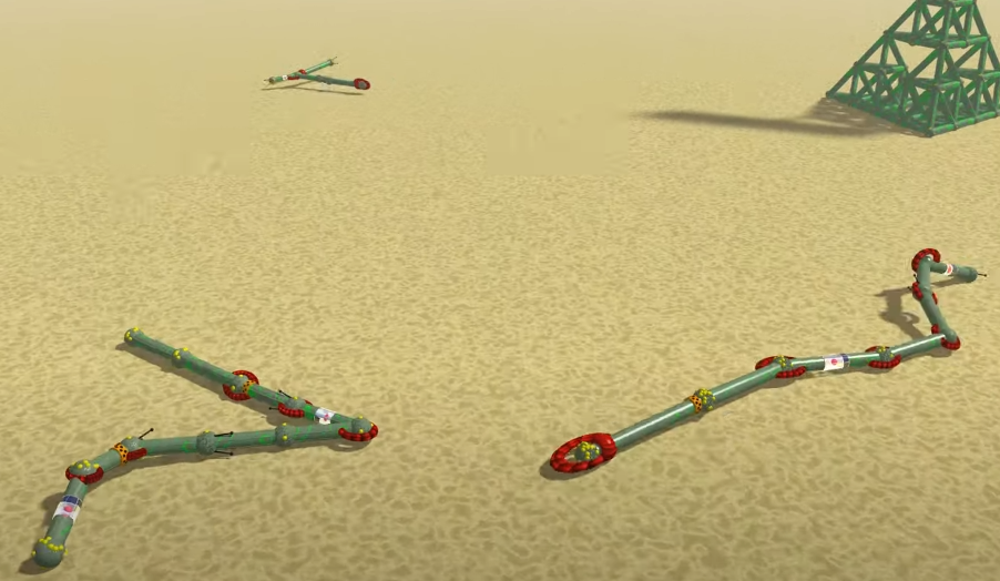
Framstick snakes 🐍
Darwin Pond
-
The previous two were physically
“realistic”.
-
Those creatures tried to resemble real creatures.
-
Darwin Pond is a bit more abstract.
-
It’s a 2D world, with only swimming physics and
restricted morphology.
-
However, it has implicit fitness!
-
There’s no hard-coded “if you find food, your
genes will pass on”.
-
The creatures that find food themselves will live on to
reproduce.
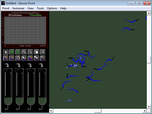
They’re making a remake of this called Richard.io.
Cellular Automata Based
-
What about something completely abstract?
-
Something that looks nothing like a creature?
-
Sure. We’ll do that next.
-
Before, reproduction was an automatic pre-defined behaviour
given by the programmer.
-
Is there a way to code the ‘physics’ of the
world to enable reproduction implicitly?
-
Sure! We can do that, with things like John Conway’s Game of Life.
-
If you don’t know what it is, it’s a big grid
of on/off cells that are either turned on or off in the next
generation based on the neighbouring cells.
-
This isn’t really evolution though.
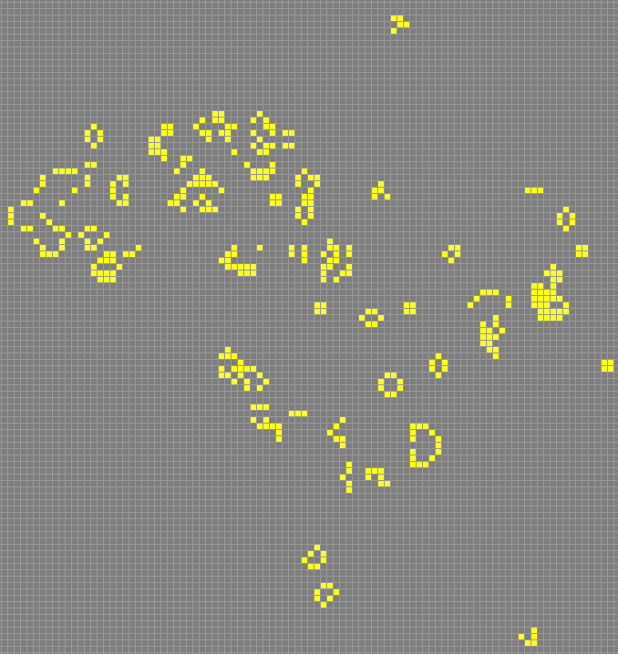
-
How about Langton loops?
-
It’s similar to Game of Life, but it’s capable
of making copies of loops.
-
So, we have reproduction, but it’s all just identical
copies of loops.
-
There’s no variation, and there’s no change in
fitness either.
-
There can’t be any variation because it’s a
completely deterministic system.

-
The last one is Hiroki Sayama’s Evoloop.
-
There are 9 states for each cell, and there are 5
neighbourhood rules.
-
There’s nothing explicit coded except those cell
rules, but it has:
-
Representation (loops)
-
Fitness (staying alive and having kids, I guess)
-
Reproduction (loops self-reproduce)
-
Variation (loops of different sizes)
-
As the algorithm goes on, you’ll see that the loops
get smaller and smaller.
-
That’s because it’s an evolutionary advantage
to get smaller, because it’s easier for them to exist (cells travel a shorter distance around the loop), and therefore, to reproduce.
At the start of the algorithm vs towards the end
-
All the properties of evolution are present, but it’s
all implicit.
-
Is that it? Have we made living things now?
-
Not quite... This is cool and all, but it’s not very
creative.
-
The individuals are just loops.
-
Can’t we implicitly evolve something that’s a
bit more expressive?
-
No, I didn’t mean loops with feelings... I meant
complex individuals.
Computer Program Based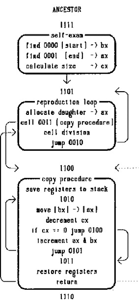
-
Tom Ray created a world called Tierra that consists of computer programs replicating
themselves.
-
They can read and write to areas of memory, and they can
copy themselves to other parts of memory and run themselves
there, called ‘forking’.
-
Random errors are sprinkled everywhere in memory at a low
rate, creating mutations.
-
There’s a ‘reaper’ that kills old
processes.
-
The first ever program in Tierra, named the Tierran
ancestor, is a simple program that replicates itself with a
copy function.
-
It’s written in an assembly-like language, so to run
its copy function, it searches for a ‘copy’
label.
-
They let it run for a while, and eventually, parasites
started to appear.
-
No, not computer viruses.
-
These parasites were imperfect copies of the ancestor with
no copy function.
-
How can it replicate with no copy function?
-
When it tries to copy, the program counter keeps
sequentially searching for a copy label until it reaches one
that’s owned by another program: a host.
-
It then uses that host to replicate, and because parasites
are much smaller, there can be more of them and can be
copied much quicker.
-
However, there must be a host for them to survive,
otherwise there’d be no copy functions to reproduce
with.
-
They let it run for a bit longer, and hosts started to
build resistance to parasites.
-
There were also hyper parasites, which were parasites that
infected parasites.
-
How does that even work?
-
I don’t know. I just write the notes.
-
So, we have implicit evolution!
-
However, it’s a bit underwhelming, don’t you
think?
-
All they make are parasites. That’s not very
fun.
-
Where’s those cool blocky box grabbers and sperm that
Karl Sims made?
-
Where’s the complexity?
-
In fact, how do we even know that evolution increases
complexity at all?
-
That’s the topic of this module, and the reasoning
behind the name Evolution of Complexity!
Arrow of Complexity
-
Does evolution naturally tend to increase the complexity of
evolved things?
|
Life on Earth is more complex now than it was
back in the primordial soup, and evolution is
the only process capable of making that
complexity, so evolution must increase the
complexity of things.
|
Evolution simply favours individuals with a
high fitness; that’s all. It doesn’t
favour complexity at all. Tierra and Evoloop
only created parasites. If evolution increased
complexity, Tierra and Evoloop would create much
more.
|
-
Who’s right? Don’t you wanna know the answer to
this burning question?
-
What?! You really couldn’t care less?
-
Tough luck, chump. It’s part of the module.
-
Let’s have a look at research regarding this
question...
-
First, how do we measure complexity?
Information Entropy
-
Information entropy: how much information there is in a signal.
-
Entropy is like a measure of how much surprise there is, or
how predictable something is.
-
Given a fair coin toss, there are two possibilities.
There’s only two options, so it’s fairly
predictable. That’s 1 bit of entropy.
-
Given two coin tosses, there are four possibilities.
That’s a bit less predictable than with one coin.
That’s 2 bits of entropy.
-
Given another coin toss, but both sides are heads, it could
be either heads or... heads. There’s no surprise there
at all. That’s 0 bits of entropy.
-
If that doesn’t make a lot of sense, check out this short video explaining it.
-
Totally predictable and ordered → low entropy
-
Totally random and unpredictable → high entropy
-
Is this a good way to measure complexity? Hmm...
Kolmogorov Complexity
-
The Kolmogorov complexity of something is the length of the shortest program (for universal Turing machines) that could generate it.
-
Therefore, the string “hello world” has more
Kolmogorov complexity than the number 6.
-
There’s a problem with this though.
-
It’s generally incomputable.
-
For example, could you calculate the Kolmogorov complexity
of:
-
An actual rainforest?
-
A Pacman frog?
-
Jonathan Joestar?
-
Richard Watson?
-
How would you even begin to generate those with a
computer?
How many lines of code would it take to
perfectly 3D model a Pacman frog?
-
Kolmogorov complexity is maximised by randomness.
-
The truly random number has the largest computer
program.
-
Entropy is also maximised by randomness.
-
A completely random 50:50 coin has the highest entropy a
coin can have.
-
We don’t want it to be maximised by
randomness...
-
We want it to be maximised by pattern, structure, or
organisation.
-
What’s the point of using a complexity representation
that says a random number is more complex than a
human?
-
Bro... you live in a world with quantum mechanics.
You’re made up of random numbers.
-
Alright, how about this?
-
If randomness is the problem, let’s say that instead
of a Turing machine, we use a sort of
‘probabilistic’ Turing machine.
-
Transitions aren’t deterministic; they’re
random instead.
-
The size of a machine to generate a random coin toss would
be tiny.
-
Therefore, coin tosses would be low complexity!
-
That’s cool I guess, but it’s still
incomputable, like with normal Turing machines.
-
I mean, we wouldn’t even be able to represent the
complexity of Richard Watson.
Structural Complexity
-
How about we go less theoretical and think more
structurally?
-
We could quantise complexity with the number of parts an
individual has.
-
What do we describe as a “part”?
-
A part could be either an object or a process (connection between objects).
-
We could also incorporate hierarchies in this
complexity.
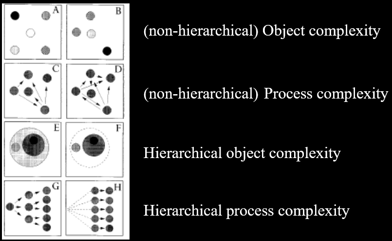
-
Hmm... maybe. We’re getting there.
McShea’s Passive Diffusion Model
-
Has life on Earth actually increased in complexity?
-
Sure, we’re pretty complex, but we still have:
-
Non-living molecules
-
Replicating molecules
- Protocells
-
Simple (prokaryote) cells / bacteria
-
Eukaryotic cells
-
Basically, bacteria that’s still not very complex
still exist in our world.
-
Why haven’t they evolved to be complex, if evolution
leads to complexity?
Yes, we still have these things in our world.
-
One explanation is that evolution doesn’t really drive complexity...
-
It just sort of happens. Some things evolve to be complex.
Some don’t.
-
You could say complexity is a result of “passive diffusion”.
-
Complex things are made, but not because complexity is
adaptive (adaptive meaning complexity is an evolutionary
advantage).
-
How do we even prove such a thing?
-
To prove this, we need to provide three things:
-
Trend: An observable increase or decrease in a measured
quantity
-
Generic Trend: robust regularity in trend (repeatable, like a ‘law’, not
accidental)
-
Mechanism: something that explains why the generic trend
happens
-
Alright, let’s set up the initial structure of our
proof:
-
Trend: complexity of life on Earth has increased
-
Generic Trend: it could be generic... who knows?
-
Mechanism: evolution, ONLY IF complexity is adaptive
-
We don’t know if this trend is generic
-
We don’t know if evolution is the mechanism, because
we don’t know if complexity is adaptive.
-
Oof.. this is pretty tricky.
-
What do the great evolutionary minds think?
-
Darwin: “from [evolution by natural selection] the production
of higher animals directly follows”
-
Dennett: complexity increase is “forced move”
-
Stephen Jay Gould: it's all ‘historical contingency’
(accidental) – passive diffusion (McShea 1994) at
most
-
John Maynard Smith: no expectation of increased complexity from natural
selection
-
Stuart Kauffman: there is a generic trend, but the mechanism is
self-organisation
-
Mark Bedau: this is all rhetoric, if you think you know a mechanism,
show me the model that exhibits the generic trend. We
haven't seen one yet!
-
Basically, Bedau says all this discussion is pointless
until someone presents a model that exhibits the generic
trend.
-
So, McShea demonstrated the “passive diffusion
model”, with the complexity on the X axis and time on
the Y axis.
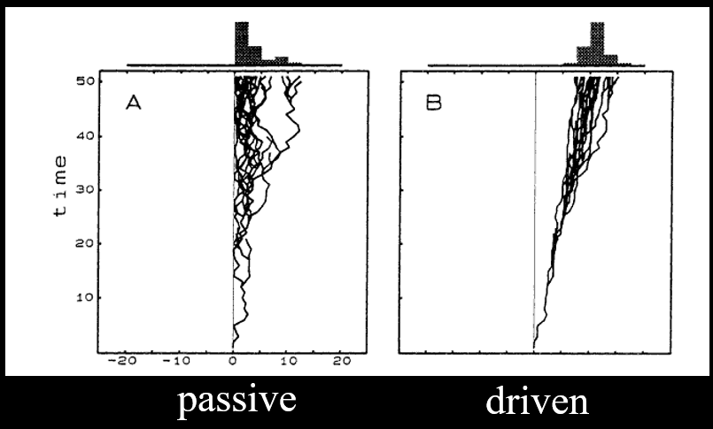
-
This graph shows that there isn’t any
“pressure” to be more complex.
-
There’s simply a distribution of individuals, with
more individuals being simple than complex.
-
Boom! That shut Bedau up.
- Or did it?
-
Well, is the X axis a reasonable dimension?
-
The X axis’ representation of complexity could be
anything:
-
Number of legs
-
Number of wheels
-
Number of pink stripes
-
This model doesn’t actually prove anything about
complexity, or produce anything complex.
-
It just differentiates between the various concepts we
might talk about.
Hierarchical Structure
-
The Tierra world from Artificial Life had all the makings
of evolution:
-
Natural selection
-
Implicit fitness
-
Infinite genetic space
-
Computational universality
-
But all it made were really small parasitic-like loops.
What gives?
-
Where’s the complexity? Where’s the loop-based
Skynet trying to take over our computers?
-
Perhaps we’re missing some “magic
ingredient”?
Tierrans with the “magic ingredient”
-
Perhaps that magic ingredient is hierarchical
structure?
-
Here are the major transitions in evolution:
-
Self-replicating molecules → chromosomes
-
Proto-cells → cells
-
Prokaryote cells → Eukaryote cells
-
Single celled organisms → multicellular
organisms
-
Asexual populations → sexual populations
-
Homogeneous populations → eusocial colonies
-
Basically, we start out as really small self-replicating
proteins from the primordial soup, and we go through stages,
or “hierarchies”, until we get to the social
human beings we are today.
-
When an organism reaches the next hierarchy, it can now
only self-replicate as part of the larger whole (e.g. when single celled organisms become multicellular, if
any more single celled organisms reproduce, that’ll
just form a bigger part of the multicellular organism).
-
Our buddy McShea from earlier, and their friend Changizi,
put these hierarchies into a graph and made sense of things
on a cellular level:
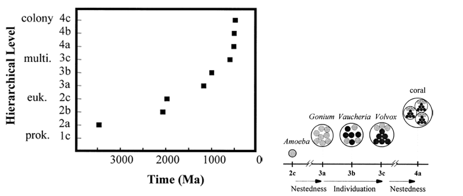
|
1) Individuals start as just a cell.
|
2) They clump together to form homogenous
organisms.
|
3) They mutate to form heterogenous
organisms.
|
4) The types of cells move apart and form
compartments.
|
5) The organisms stick together and form
colonies.
|
|

|

|

|

|
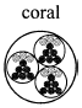
|
-
The different degrees of individuation are:
-
Monomorphic aggregate
-
Differentiated aggregate
-
Differentiated aggregates with intermediate level
parts
-
This hierarchical evolution is pretty cool...
-
Maybe it really is a generic trend.
-
However, standard models of EA don’t support this
kind of hierarchical organisation.
-
Plus, nobody has demonstrated a generic trend for
hierarchical complexity in artificial life models.
-
Back to the drawing board...
-
If increases in complexity really is a generic trend,
what’s the mechanism that causes it?
-
If evolution really does increase complexity, what are we
missing in our current models?
-
Is it any of these?:
-
Rich physical environment
- Coevolution
-
Self-organisation
-
Dynamical systems theory
-
Mechanisms of encapsulation
- Hierarchy
-
Changes in the unit of selection
Natural Induction (not examinable)
-
Apparently, this section is not examinable, so read this if
you’re interested.
-
In addition, I don’t fully understand natural
induction, so I’m giving a very brief abstraction of
what natural induction is.
-
Please correct anything if it’s wrong!
-
In a population, we have a fitness landscape.
-
We want our individuals to be at the dips of the landscape (minimising function), because that means they have the highest fitness (lowest cost) they can have.
-
Thing is, they usually don’t go to the highest
fitness levels.
-
Individual hill-climbers are selfish, and only remain on
local optima that maximise their individual utility.
-
If these hill-climbers were to work together and
collaborate, they could probably reach higher maxima.
These graphs will be minimisation functions, not
maximising.
-
They don’t want to work together because that
won’t maximise their individual utilities.
-
They need to be part of a ‘social organisation’
where they work together for the greater good.
-
So how do we cause individual incentives to become better
aligned with social incentives?
-
How do we make “working for the greater good”
also benefit individual utility?
-
We use natural induction!
-
First of all, what is induction?
-
Induction is the production of general rules from specific
examples.
-
Some examples are:
-
This colourful thing tastes good 🍓
-
That colourful thing taste good 🍩
-
Therefore all colourful things taste good
🍓🍩🍌🍊🍬🍭🍫
-
Or mathematical induction:
-
The sum of natural numbers up to 1 is

-
The sum of natural numbers up to n + 1 is

-
Therefore the sum of natural numbers up to any n is

-
There’s even an example on Richard’s
T-shirt:
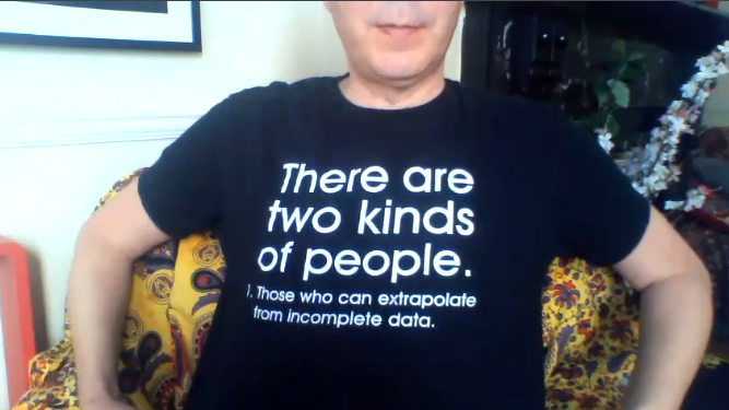
-
Of course, induction isn’t always logically
sound.
-
It’s just the idea behind the concept of natural
induction.
-
Natural induction is a process by which a dynamical system becomes adaptively
organised spontaneously.
-
It doesn’t require natural selection, or some kind of
system-level objective function.
-
There’s three requirements for natural induction to
occur in a dynamical system:
-
Hidden state - interface variables and internal state
-
Imperfect elastic interactions
-
PULSE - repeated exposure to stress or perturbation
-
If that makes no sense, read on: I’ll try and make
heads or tails of it.
|
What is ‘hidden state’?
|
|
Let’s go back to our minimisation
function example.
Let’s say we have an individual
that’s stuck on the landscape
somewhere.
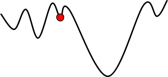
From all our previous examples of individuals
travelling across the fitness landscape, our
individual is stuck in that local optimum
dip.
But what if we could change the
individual’s perception of their utility function?
In other words, all the individuals have their
own mutable, shared “copy” of the
fitness function that they travel across?

We could change the individuals’
perception of their utilities to travel up peaks
they normally wouldn’t want to travel
across!
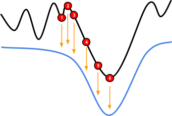
This blue ‘perception’ of the
utility function is the hidden state; it’s
an invisible force that drives the variables we
can see (namely, the individuals), and it’s called hidden state because we can change it.
|
|
What is ‘imperfect elastic
interactions’?
|
|
How much do we want to change our hidden
state?
If the hidden state is too rigid, it
won’t change at all, and there’d be
no point having it.
If the hidden state is too plastic-y,
it’ll be like clay and change too
much.
|
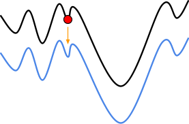
It’s not changing, so
we’re not moving
anywhere.
|
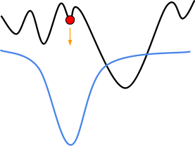
I didn’t want to change
it that much!
|
We want a sweet spot.
We want to be able to change our hidden state;
not so rigid that we can’t budge it, but
not so soft that there’s zero resistance
and it goes everywhere.
That’s what we mean by ‘imperfect
elastic interactions’.
If this is a little hard to visualise, think of
it like this:
|

|
|
|
|
Steel pole: impossible to bend. Too
rigid.
|
Wet spaghetti: always falls out of shape.
Too soft.
|
Copper wire: it’s malleable enough
to bend, and it’s tough
enough to retain its shape.
Nice! We want our hidden state
to be like this.
|
|
|
What is ‘PULSE’?
|
|
So we have a hidden state that lets us control
where the individuals go as a group, and we can
bend it to our will.
But what do we change the hidden state
to?
Onto that in a second! First, let’s
define what we mean by
‘PULSE’.
Do you remember simulated annealing from Intelligent
Systems? If not, it’s about using temperature to
‘scramble’ the individuals to escape
local optima.
|
Big β, low
temperature
|
Small β, high
temperature
|
|
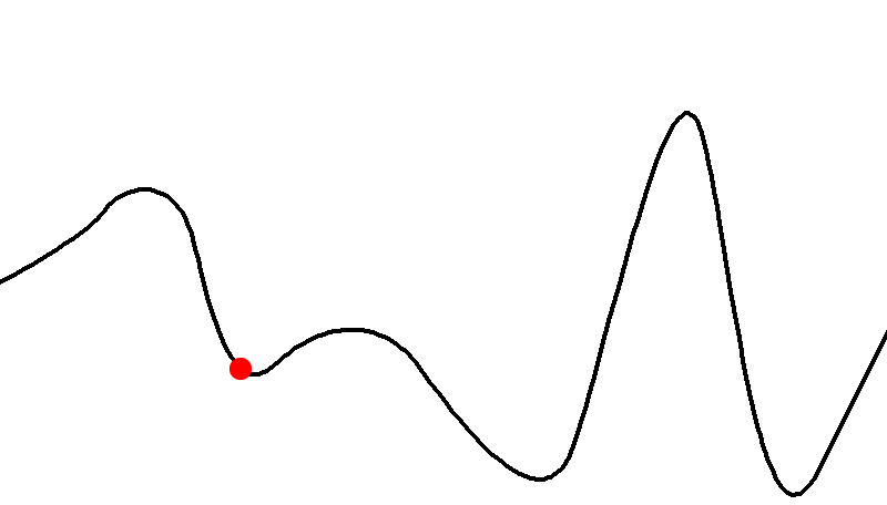
|

|
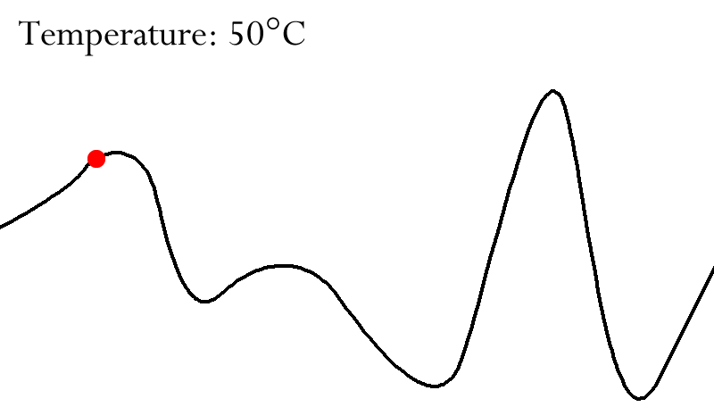
That’s pretty much what PULSE is.
It’s the ability to ‘heat up’
individuals and make them scatter about to find
other optima.
|
-
Great, so how do these properties result in natural
induction?
-
Remember when I talked about increasing the heat of the
population?
-
When we do that, the individuals will, on average, evenly
fall all across the fitness landscape.
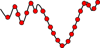
-
Because they all fall evenly, they form a
‘distribution’ of all the local optima in this
landscape.
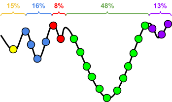
-
The distribution of the optima affects how much the hidden
state is ‘pushed’ at each point in the landscape
by the individuals.
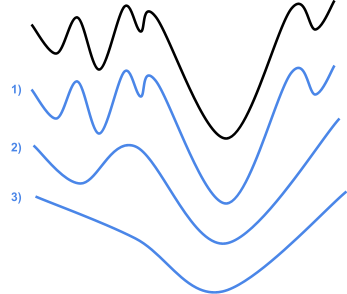
-
Then, the individuals are heated up again and the cycle
continues.
-
As this continues, the dips with the wider basins get
greater and greater prevalence in the hidden state, so
individuals land in the dips with the wider basins
more.
-
Now, we’ve pushed the hidden state so much that
there’s only one really big dip.
-
That big dip drives all the individuals to the global
optimum.
-
You see? With the power of teamwork, all the individuals
explored the fitness space, and drove the hidden state in
such a way that the global optimum came out on top and drove
out the smaller local optima.
-
That’s a super simplified explanation of natural
induction.
-
If you’re:
- Masochistic
-
Richard Watson
-
Want to do a PhD with Richard Watson (a.k.a the first point)
Compositional Evolution
“If it could be demonstrated that any complex organ
existed which could not possibly have been formed by numerous,
successive, slight modifications, my theory would absolutely
break down.” - Darwin, 1859
-
Hmm... could we?
-
In more detail, Darwin says that every individual evolved
through the succession of many ‘proto-systems’
that are gradually increasing in function.
-
Proto-systems are intermediary creatures in the evolutionary
process that lead up to a more complex creature, like you or
me.
-
We will show that it’s possible to make creatures
without proto-systems, but that doesn’t mean
Darwin’s theory is wrong.
-
Are proto-systems required?
-
Proto-systems leading up to complex individuals are a
result of natural selection.
-
That means creating a new individual based on variation and
whoever here has the highest fitness.
-
But there’s other ways to make new individuals:
-
Sexual recombination / hybridisation
-
Uniform crossover, one-point crossover etc.
-
You can get really big genetic changes in one step, unlike
mutation.
-
Genes are transferred across species barriers.
-
For example, a bacteria transferring antibiotic resistance
genes to other species of bacteria through either transformation, transduction, or conjugation.
-
This is mostly done by bacteria.
-
One organism merging with, and becoming a part of, another
organism.
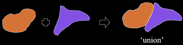
-
The hierarchical major transitions I mentioned back in
Arrow of Complexity.
-
Self-replicating molecules → chromosomes
-
Proto-cells → cells
-
Prokaryote cells → Eukaryote cells
-
Single celled organisms → multicellular
organisms
-
Asexual populations → sexual populations
-
Homogeneous populations → eusocial colonies
-
These ways of making individuals is less about mutating an
existing individual, but about putting two individuals
together to make a new individual.
-
We call this compositional evolution.
Gradual vs Compositional
-
Compositional evolution doesn’t use proto-systems,
but are still capable of evolving life, like Darwin
thought.
-
Therefore, a succession of gradually changing
proto-systems, monotonically increasing in function, is not required for evolvability of certain kinds of complex
systems.
-
Let’s look into this a little deeper:
-
Driven predominantly by small modifications, hence
‘successive slight modifications’.
-
Individuals are reached by linear accumulation of random
variations.
-
Variation → genetic mutation
-
Evolution that involves the combination of pre-evolved
systems or subsystems of genetic material that were
pre-adapted in different individuals.
-
Variation → sexual recombination, horizontal gene
transfer, symbiogenesis
-
On a fitness landscape, you can think of gradual evolution
as like a hill-climber:
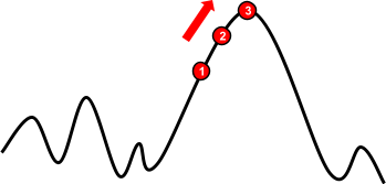
-
You can think of compositional evolution as two individuals
forming a new individual on a completely different
landscape:
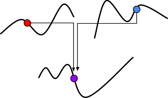
-
How about on an evolutionary tree?
-
One with time on the Y axis and variation on the X
axis.
-
Gradual evolution looks like this:

-
Simple enough. Everything starts at a common ancestor (the root), and through time, the variation of individuals changes,
and species branch off.
-
How about compositional evolution?
-
Well, what do Doolittle and Margulis think?
|
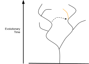
|
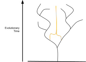
|
|
Doolittle
|
Margulis
|
-
They’re both not exactly right.
-
With Doolittle, it seems like individuals from one branch
are “becoming” individuals from another branch.
That’s not quite right; we’re making a whole new
individual altogether.
-
With Margulis, it looks like the two species keep evolving
until they both evolve into the same thing. That’s
also not right, because they’re meant to merge; not
meet in the middle.
-
In reality, it should look like this:
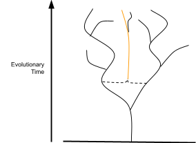
-
Here, two individuals form a completely new
individual.
-
subdivisions are subpopulations in a species
-
integration is done by sexual recombination
-
Examples:
-
Shifting Balance Theory (Wright 1931)
-
Building Block Hypothesis (Holland 1975)
-
In symbiotic encapsulation,
-
subdivisions are different species
-
integration is done by horizontal gene transfer and
endosymbiosis (bacteria going inside, and becoming a part of, a host
cell)
-
Examples:
-
Major evolutionary transitions
-
Problem decomposition by coevolution
Complex Systems
-
The different kinds of dependencies between variables can
affect the system in various ways:
|
Dependency of variables
|
Arbitrary interdependencies
|
Modular interdependencies
|
Few / weak interdependencies
|
|
Landscape
|
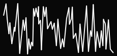
|

|

|
|
Algorithmic paradigm
(what algorithm to use?)
|
Exhaustive search
Random search
|
Divide and Conquer problem decomposition
|
Hill-climbing - accumulation of small
variations
|
|
Complexity
|
KN
|
Nk
|
KN
|
|
Evolutionary analogue
|
Impossible / ‘intelligent
design’
(it’s virtually impossible to make an
evolutionary algorithm find a global optimum in
this)
|
Compositional evolution
|
Gradual evolution
(need to find small paths)
|
-
Could we come up with a problem that can be solved with
compositional evolution, but not with gradual
evolution?
-
It needs to have the elements that make it hard for gradual
evolution:
- Ruggedness
-
Lots of local optima
-
Broad fitness saddles
-
It needs to have the elements that make it easy for
compositional evolution:
- Modular interdependency
-
Subsystems that can be solved independently and
combined
-
Epistasis prevents linear accumulation of subsystems
-
How about the HIFF function we looked at back in
Modularity, to show that there exists a problem that
crossover can do better than a hill-climber?
HIFF
-
If you forgot, HIFF looks like this:
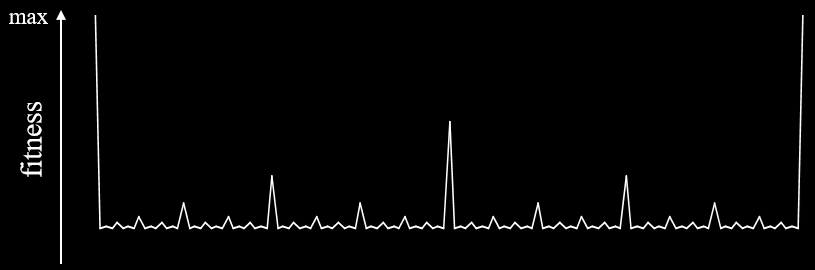
-
It’s specially designed so one-point crossover can
solve it really quickly, but hill-climbers cannot.
-
If hill-climber relates to gradual evolution, and crossover
relates to compositional evolution, won’t the latter
be better than the former at HIFFs?
-
Here’s a graph:
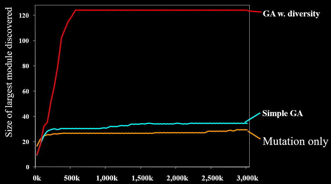
-
Yep! GAs with one-point crossover are way better.
-
So compositional evolution is way better at HIFFs than
gradual evolution.
-
But we already know that from Modularity.
-
How about we make the problem slightly more complex?
Random Genetic Map and SEAM
-
Before, we assumed that all modules are located together on
the genome.
-
Not all real-world problems are going to have a convenient
genome like that.
-
What if we scrambled the locations of the modules?
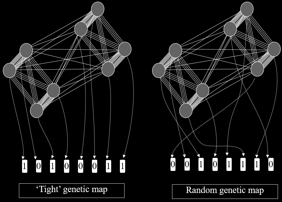
-
How do the algorithms fare now?
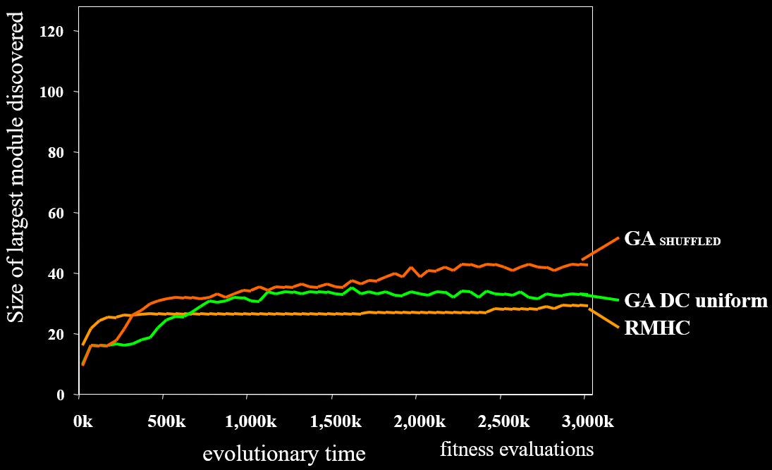
- Oof...
-
We need an algorithm that not only uses compositional
evolution, but also identifies modules regardless of
location on the genome.
-
Introducing SEAM!
-
SEAM uses coevolution of different individuals to cover
different parts of the problem space.
-
When it finds a successful group (in other words, a permutation of loci that behave very
‘modular’), it encapsulates that and remembers it.
-
That’s called symbiotic encapsulation.
-
In a more general sense, it finds the modules with
permutations of loci, and then evolves using that in
mind.
-
How well does SEAM perform?
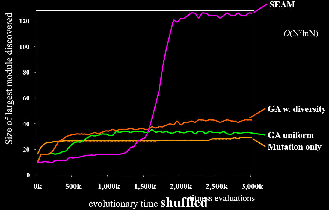
-
That looks good!
-
It’s low at the start because it’s still
learning where all the modules are.
-
Once it knows, it performs just as well as a one-point
crossover GA.
-
This makes SEAM really good for:
-
Divide and conquer with compositional evolution
-
Evolving parts and putting them together
-
The only problem is that it’s only good for
HIFF.
-
A problem that we invented.
- 🙃