OSI model	TCP/IP model	Tanenbaum’s book
Application	Application	Application
Presentation	Transport	Transport
Session	Internet	Network
Transport	Link	Link
Network	Hardware	Physical
Data Link
Physical

Here is a sentence to remember the OSI layers, from bottom up: Please Do Not Throw Salami Pizza Away 🍕❌🗑

Tanenbaum’s book is just the TCP/IP model, but they changed Internet to Network and Hardware to Physical.

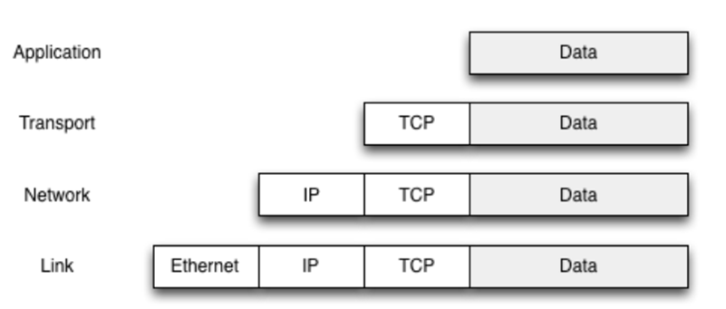
Each layer adds its own header, and it becomes part of the payload for the layer below it:

There’s different types of medium for the physical layer:

Coaxial cable
Twisted pair
Power line
Fibre optic
Wireless (laser, sound, ultrasonic, pulses, radar)

Bits are transmitted using encoding schemes. Transmission is based on something varying over time, like voltage or frequency, with synchronisation.

What does the link layer actually do?

Transmits frames over physical media
Detects and handles transmission errors

The link layer doesn’t care about what the packet says. The link layer only cares about getting the packet from A to B.

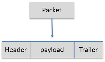
Packet: a unit of data in the Network layer (our payload)
Frame: a unit of data in the Link layer (what the link layer actually sends)
A frame contains a packet and wraps a header and a trailer around the packet.

Data frames vary based on the physical layer, for example there are Ethernet frames and Fibre Channel frames.

The partitions of a frame are usually fixed in size (except for the payload), making it far easier to tell where the data actually is.

Frames are transmitted through hop by hop transmission over a packet-switched network.
Too jargon-y for you?

Hop by hop transmission: where data is transported through intermediate nodes to its destination.
Packet-switched network: A network where packets dynamically find their own way to a destination without a set path (look at the pretty animation from wikipedia)

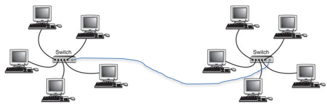
Because of these properties, framing can allow senders to send packets through a shared medium, like you see above (all the intermediate nodes are available to all the coloured packets/frames).
You also need to know where the frame starts and the frame ends.

In flow control, we may need to regulate how fast we send data. We don’t want to swamp a slow receiver with tons of packets!
We can either:

send messages from the receiver to the sender saying “wait, let me process this data first” and alternatively, “alright, now send more data” a.k.a. feedback-based flow control
make the communication rate-based so the speed is agreed between both parties (rarely used in such a low layer) a.k.a. rate-based flow control

Acknowledgements

There are three main link layer models:

Connectionless, no acknowledgements

Used for low error rate networks (networks where packets rarely get lost, like Ethernet)
Connectionless: no signalling path is established in advance.
No acknowledgements: Frames are sent, and may or may not be received by the destination.

Acknowledged, connectionless service

Acknowledged: frames are sent, and the recipient notifies the sender when they’ve received a frame through an acknowledge (ACK) signal.
This is used when connections need the assurance of delivery, but can’t afford the overhead of connection management.

Acknowledged, connection-oriented service

Acknowledgement signals are sent, and a connection is formally established before communications occur.
This is used for long delay, unreliable connections, for example with satellites.
It’s computationally expensive, but it’s secure.

How do we handle ACK signals and errors?
We use ARQs!
ARQ (automatic repeat-request): an error-control mechanism that uses ACKs and timeouts to ensure reliable communications with an unreliable recipient.
Basically, ARQs are different ways of handling ACKs and when they screw up.
There are three kinds:

ARQ protocol name	Explanation (not in the slides, so it might not be examinable, but if you wanna play it safe then read this anyway)
Stop-and-wait	The sender sends the first frame, then the recipient sends an ACK signal for that frame. The sender sends the second frame, then the recipient sends an ACK signal for that frame. This keeps on going until all the frames have been sent.
Go-back-N	The sender sends frames #1 to #N to the recipient, in order, over and over again, even if an ACK signal doesn’t exist. The recipient throws away duplicate frames and frames that aren’t in the right order. The recipient sends an ACK signal containing the lowest number frame it had missed, let’s say #M where 1 ≤ M < N. The sender gets the ACK signal, and now sends frames #M to #(M + N) to the recipient. This keeps on going until all frames are collected. Protocols like these are called sliding window protocols. Example: Alice is sending frames 1, 2, 3, 4 and 5. Bob gets frames 1, 2, 3 and 5, but misses 4. Bob sends an ACK signal to Alice with the number ‘4’. Alice receives this ACK signal, and is now sending frames 4, 5, 6, 7 and 8. Now Bob has frames 1, 2, 3, 4, 5, 6, 7 and 8. Bob sends an ACK signal with the number ‘9’. Alice receives this ACK signal again, and is now sending frames 9, 10, 11, 12 and 13.
Selective-repeat	Go-back-N may send duplicate frames, which is inefficient on the bandwidth. Selective-repeat aims to fix this. The sender sends frames #1 to #N. The receiver can either: Send an ACK signal to move onto the next set of frames Send a NAK signal to request a specific frame If the sender gets an ACK signal with number M, then it’ll start sending frames #M to #(M + N). If the sender gets a NAK signal with number M, then it’ll send only the frame #M to the recipient. Example: Alice sends frames 1 and 2 to Bob. Bob gets frames 1 and 2, and sends an ACK signal with number 3 to Alice. Alice gets this ACK signal and sends frames 3 and 4 to Bob. Bob misses 3, but gets 4. Bob sends a NAK signal with number 3 to Alice. Alice gets this NAK signal, and sends frame #3 to Bob. Bob gets frame 3 and sends an ACK signal with number 5 to Alice. Alice gets this ACK signal and now sends frames 5 and 6 to Bob.

How do we detect errors in communication?
There are a few ways we can do this:

Parity bit: a bit that’s either 1 or 0 depending on whether the number of 1’s is even or odd
CRC (Cyclic Redundancy Check): a type of checksum based on polynomial division. The checksum is stored in a field of the frame, and is calculated and compared by the sender and the recipient.

Checksums may happen on other layers too. IPv4 has a checksum, but IPv6 doesn’t.

Frames

In frames, how do you know where frames start and where frames end?
There’s many ways to do it. One way is to use a FLAG byte value to mark the start and the end.
If a FLAG byte appears in the payload, escape it with an ESCAPE byte (similar to escape characters \n, \b, \\ ... in C, C++, Java etc.)

Ethernet CSMA/CD

Ethernet was the de facto link layer standard throughout the 90’s, and continues to be today.
Originally, it all ran through shared media. In other words, it was all one wire and everyone had to share. There came twisted pair with hubs/repeaters to help, but it didn’t solve the problem.
In the end, switches were used (they’re like hubs, but a little smarter). There is one device per switch port, and since it’s fully duplex, there’s no contention.

On a shared medium, how is media contention handled?
Originally, Ethernet used Carrier Sense Multiple Access with Collision Detection, or CSMA/CD.
It works by checking if the media is busy. If it is, then wait. If it isn’t, then it sends its signals across it.
If a collision occurs (two devices try to use the media at the same time), they both stop and pick a delay before trying to talk again.
Ethernet doesn’t really use this anymore because switches are fully duplex, so there’s no contention.

WiFi CSMA/CA

WiFi is the wireless alternative to Ethernet. It works in the 2.4GHz or 5GHz range. The 2.4GHz range has 14 channels (13 in Europe). WiFi has evolved over the years.
With WiFi, devices are associated with a wireless access point (AP). Devices can select from one of many service set identifiers (SSIDs).
WiFi is technically a shared medium, so there can be contention in a busy area. Therefore, you need a collision avoidance scheme.

WiFi can’t send and receive at the same time, so WiFi uses a slightly different approach called CSMA/Collision Avoidance (CSMA/CA).
It’s like CSMA/CD, but instead of listening to the medium, it waits for an acknowledgement from the AP to determine if the frame was sent.
In other words, instead of dealing with collisions, it avoids them.
It’s very similar to the stop-and-wait ARQ protocol.
Optionally, Request to Send / Clear to Send (RTS/CTS) could be used to improve performance, where a sender sends an RTS message to ask if it can send frames, and can only send frames after it receives a CTS message from the receiver (basically, send an RTS and expect a CTS).
/CA is used in wireless connections as it is very difficult to determine if a collision has occurred over a wireless network.

Ethernet LANs

Ethernet theory

Ethernet is used on campus networks and on home networks.

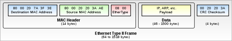
An Ethernet frame includes (remember, this is the link layer):

48-bit source MAC address
48-bit target MAC address
Optional VLAN ID and frame priority

At max, the frame is usually around 1500 bytes. If it gets any bigger, it’ll be broken down into smaller frames.

MAC (Media Access Control) address: a unique ID for network interface controllers (NICs) at the link layer.
It’s around 48 bits long, but can be extended to 64 bits.
They need to be unique, so MAC addresses are split up into:

24 bits for vendor allocations (tells you what vendor this hardware is from)
Last 24 bits assigned by the vendor

Ethernet networks are built with each device (also called hosts) connected to a concentrator device (usually a switch).

Desktops usually have 1 Gbit/s Ethernet, but the servers are on 10 Gbit/s Ethernet.

There are different kinds of concentrator devices:
Hubs and repeaters:

Really old!
They just take frames and forward them on to all the devices available
They just extend Ethernet range
All hosts see all packets, which is a big no-no for security.

Bridges and switches:

Receives frames and forwards them to the host that needs them
Has ‘smart’ forwarding (they learn which host needs what packet)
Hosts only see the packets sent to them, which is good for security.
Switches are smart, because:

they can perform CRC (Cyclic Redundancy Checks) before forwarding
it learns the addresses of the hosts using a MAC table, so they only send packets to the hosts that need them
can support more advanced features, like VLAN or QoS

How do switches learn which frames go to which host?
Switches match up source MAC addresses to switch ports.
So if a frame with source MAC address 6F-72-61-6F-72-61 is picked up by port number 2, the switch will remember that. The next time a frame with that source MAC address comes up, the switch will send it to port number 2.
There is a time-out for pairings like that (~ 60 seconds).
If there is no entry in the table the switch has to send the package to all ports.

ARP

To send a frame to a host, you need its network layer address (IP address) and its link layer address (MAC address).
We can get the IP address from DNS, but how do we get the MAC address from an IP address?
We use ARP!

ARP (Address Resolution Protocol): a protocol that allows a host to get the MAC address associated with a given IP address.
ARP uses a link layer broadcast message (a message sent to everyone).
The broadcast message asks “Who has this IP address”?
All the hosts see this message, and the one with that IP address goes “It’s me! My IP address is so.me.th.ing and my MAC address is wh:at:ev:er”
The sender gets this information and can now send the frame.
This information is usually cached for around 60 seconds.

In an ARP message, you have:

Sender MAC address
Sender IP address
Target MAC address (zero-padded when we don’t know what it is)
Target IP address

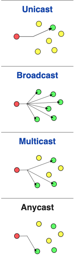
There are 4 kinds of messages:

Unicast: from one sender to one receiver. Purely one-to-one.
Broadcast: sent to everyone. To broadcast a message, make the MAC address FF:FF:FF:FF:FF:FF.
Multicast: sent to anyone who is interested.
Anycast: sent to the nearest receiver; doesn’t matter who, as long as it gets to someone.

Nuances of ARP:

Hosts can spoof and steal frames from other hosts
Low power devices may ‘sleep’ and not respond to ARP messages
You can send a ‘gratuitous ARP’, which is just making sure your information is up to date.
ARP probe: a use of ARP to make sure no two hosts have the same IP

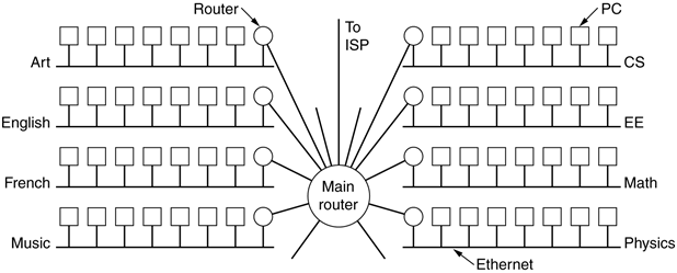
Building Ethernet LANs

LANs can’t be too big, or else we’ll have problems with range and volume of messages (when broadcasting).
Therefore LANs must be kept at a reasonable size, for example in a campus, there’s typically one LAN per floor, or per building.

When we create an Ethernet LAN with a switch, hosts can talk to each other directly using their MAC addresses.
They’ll also allocate “local” IP addresses to each host, for example 192.168.0.0 up to 192.168.255.255, as part of an IP address plan.
To connect two LANs together, we need to use an IP router, which forwards IP packets between LANs (remember, routers do not work with the link layer, only the network layer).
Routers can tell other routers the reachability of the IP address ranges it serves, so the network can learn where to forward IP packets.
Therefore, if a host was sending a packet from one LAN to a host on another LAN, it will send the packet to its ‘default’ IP router.

IP routers act as network layer gateways between individual link layer Ethernet LANs.
A localised network layer LAN behind a router is called an IP subnet.
A home network is usually a single IP subnet and Ethernet LAN.

In multi-story buildings, they typically use copper twisted pair cabling.
Ethernet networks may be deployed using:

Data riser: vertically aligned switch/server rooms
Flood wiring per floor: have faceplates from switch room
Ethernet switch stacks: one switch port per faceplate

A building may have one LAN, if a router connects the whole building, or there could be one LAN per floor.

In homes, you typically have an ADSL router with multiple Ethernet ports and 802.11 WiFi. It’s just one LAN, with no internal routing. Pretty basic.

Spanning tree protocol

A bridge loop occurs in a network when there are two ways to reach the same node.
They’re bad news because they can cause broadcast radiation, which is where there’s so much traffic on the network cabling that it severely harms the performance of the network.

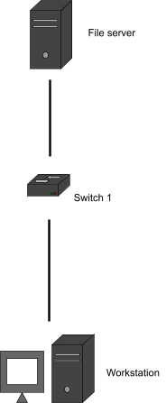
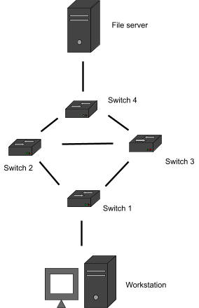
No bridge loop	Bridge loop

Why is this so bad?
Let’s say the workstation wants to send a frame to the file server. The switches will pass the frame onto the neighbouring nodes, right? After all, no frame has been sent before, there’s no way the switches would know which frames to send where.
The workstation’s frame could end up back at switch 1 through the path 1 -> 2 -> 3 -> 1 or 1 -> 3 -> 2 -> 1. This loop is wasteful and clogs up the medium.
The file server could also end up with two of the same frame.

It’s pretty clear that loops are bad. But they could also be good, because what would happen if switch 3 dies? We could still use the switch 2 path to get to the file server. Whereas, on the left, if switch 1 dies, that’s it. No more talking to the file server.

Introducing the spanning tree protocol!
The spanning tree protocol maps out a set of paths from the source to the target in a “tree” structure. It plucks out the least cost path, and disables all the other switches that are not on that path.
The source can then send the packet, and no loops will occur.
However, if a switch on that path fails, the protocol will pick the next best path, and re-enable and disable the appropriate switches to follow that path instead.
Therefore, we get the best of both worlds: no broadcast radiation, and if any switches fail, we’re fine.

Want an example?
So we want to get from the workstation to the file server. There’s two (sensible) ways of doing this:

Normally, we’d pick the smallest, but they’re both the same length, so let’s go with the switch 3 path.
So now, switch 2 is disabled. The workstation sends the frame.
Oh no! A rat chewed on the cabling of switch 3 and made it explode! What are we going to do?!
The protocol will now pick the switch 2 path. So now, switch 2 is enabled, switch 3 is “disabled”, and the frame is re-sent through the switch 2 path.
It reaches the file server successfully!

VLANs

A VLAN, or a Virtual LAN, are broadcast domains that are partitioned and isolated.
A VLAN can consist of multiple hosts, all of different LANs, but they are made to think that they are all connected to the same wire.
Ethernet frames include an optional VLAN identifier. It’s 12-bits, so there are 4096 different VLAN IDs.
Because it’s completely logical and not physical, it’s quite flexible.

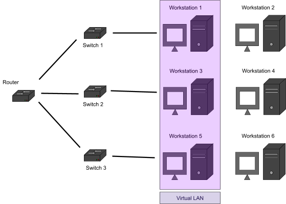
Here, workstations 1, 3 and 5 think they’re all on the same LAN, but really it’s a VLAN.
This is useful to group together staff that aren’t physically in the same LAN, for example, workstations 1, 3 and 5 might all be in the marketing department.

Ethernet frame priority

How important is a frame?
VoIP is pretty important, because you want to know what the other person is saying as they’re saying it.
HTTP might not be as important, because it’s a document; you don’t need it right away.

There are three bits in the 802.1Q tag that determines priority, from 1 to 7.
This only affects prioritisation at switches, not end-to-end.

Internet/Network layer

What does the network layer actually do?
The network layer is responsible for establishing a network between computers so that they can send things to each other.
In more detail, the network layer is responsible for:

Internetworking:

Connecting networks together to form an “internetwork”, or “Internet”
Each network is served by a router

Transmitting:

Packets the data by adding an IP header
Processes and routes IP datagrams (data units across the network)
Fragmenting packets that are too big

Receiving:

Error checking
Reassembling fragments if needed

Internet Protocol (IP)

IP (or Internet Protocol) is the main protocol used in the network layer.
The properties of IP are:

Packet-switched, connectionless:

IP packets are routed towards destination at each router on the path
Connectionless: packets find their own way to the destination, it doesn’t have to rely on a fixed path from A to B

Unreliable:

No guarantee that any IP datagram will be received
Best-effort delivery: there is a variable bit rate and latency and packet loss depending on the current traffic load. Basically, the routers try their best but won’t guarantee perfect performance

Routing:

Sending a packet is only based on destination IP address
Routers maintain routing tables to make routing decisions

Globally unique, delegated addresses:

Devices must be globally unique + addressable to send traffic to them
Private address space, which are not globally routed, may be used (because that’s the whole point, since we ran out of IP addresses)

There are 5 main protocols for the network layer:

IPv4
IPv6
ICMP - used for diagnostics and control
ICMPv6
IPSEC - used for security

Store-and-forward packet switching is a technique where data is sent to an intermediary node and then passed on to either another intermediary node or the destination node.
In this context, routers store the packet and determine where to forward them.

IP is a bit unreliable, because routers forward packets on a ‘best effort’ basis.
Packets may get dropped because of congestion. The transport layer (next layer above) may handle retransmissions:

With TCP, retransmissions are handled
With UDP, the application layer has to handle retransmission

Quality of Service may help by prioritising certain traffic.

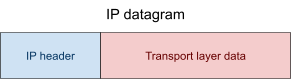
In IPv4, segments of data are taken from the transport layer and an IP header is attached to the end of it.
This creates an IP datagram.

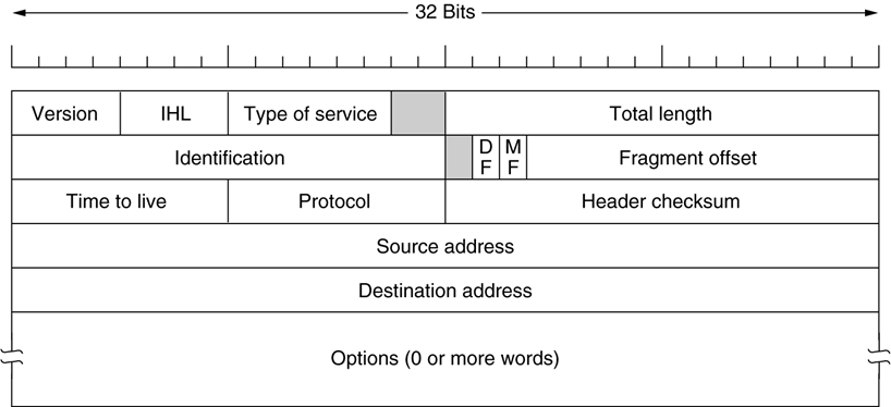
An IP header has the following fields:

Source IP address
Destination IP address
IHL - header length (can vary)
Identification field and fragment offset
Time to live (how long should this packet stay switching before we give up)
IP header checksum

MTU (or Maximum Transmission Unit) is the size of the largest data unit that can be communicated in a single network layer transaction.
If we’re sending a packet of 2000 bytes to a router, and the MTU is 1500 bytes, then the packet has to be fragmented.
Fragmentation happens in the network layer.
We should try to avoid fragmentation, because it adds overhead and security issues.

Now, a bit of history of IPv4!

People used IPv4 since the 1970’s
It uses 32-bit addresses, written as ‘dotted quads’, like 152.78.64.100.
The IPv4 address space is partitioned into 5 different classes, where 3 classes are used for networks of different sizes, 1 class is used for multicast groups and 1 class is reserved:

Class	Prefix range	Prefix length	# of networks	# addresses per network	Examples
A	0.0.0.0 to 127.0.0.0	8 bits	128 networks	~16 million addresses	20.xx.xx.xx 102.xx.xx.xx
B	128.0.0.0 to 191.255.0.0.	16 bits	~16,000 networks	~65,000 addresses	152.78.xx.xx 160.125.xx.xx
C	192.0.0.0 to 223.255.255.0	24 bits	~2 million networks	256 addresses	196.50.40.xx 202.155.4.xx
D	224.0.0.0 to 239.255.255.255	n/a	n/a	n/a	n/a (used for multicast groups)
E	240.0.0.0 to 255.255.255.255	n/a	n/a	n/a	n/a (reserved)

Here is a graphical visualisation of the partitioning of the IPv4 address space:

Class A	Class B

	Class C	Class D
		Class E

Basically, if an IPv4 address is within a certain class, it must follow two rules:

The first 8 bits must be within a certain range
It must have a fixed prefix

For example, if an IP is within class B, the first 8 bits must be between 128 and 191, and the first two bytes must be fixed.
Additionally, an IP range of 152.xx.xx.xx cannot be within class A because the first byte lies outside of A’s range; it would be B, but the second byte would be part of the fixed prefix too, so you should write something like 152.78.xx.xx.

This is generally very inefficient, e.g. there are not many networks that require a Class A IP address and thus 16 million different addresses, which means that a lot of space is wasted. Even 65,000 addresses in class B are too many for most networks.

Since 1995, RIR (Regional Internet Registry) allowed variable length prefixes, meaning that network addresses were no longer assigned strictly based on the ABC class scheme
This change reduced address consumption rate, but we still ran out of addresses back in 2011.

Due to the fact that there are still not enough IPv4 addresses for all hosts world-wide, private IP addresses were introduced
More precisely, there exist ranges in the IPv4 address space that are used as private IP addresses
What does private IP address mean? It basically means that this is an IP address that is not globally unique and thus cannot be reached from outside the network.
In other words, private IP addresses may be used many many times in different networks world-wide
An example for the use of a private IP address is your home network
There exist three different private IP networks with the following address ranges:

Address range	Number of addresses	Subnet mask
10.0.0.0 - 10.255.255.255	16,777,216	8 bits mask
172.16.0.0 - 172.31.255.255	1,048,576	12 bits mask
192.168.0.0 - 192.168.255.255	65,536	16 bits mask

For example, your home network may use 192.168.0.0
You can further divide the private address space into subnets as you wish (more on subnets later), so you could have 192.168.0.0/24, allowing for 255 ip host addresses
There must be a mechanism to translate your private IP address to a public ip address, which is called NAT (see below)

We can maximise the use of address space:

DHCP (or Dynamic Host Configuration Protocol) requires IP addresses to be leased out for small time periods, preventing inactive hosts from hogging valuable address space
NAT (or Network Address Translation) allows you to use one IPv4 address to refer to an entire private network, so each device on your network doesn’t need their own unique IPv4 address
Classless Inter-Domain Routing: allows use of any prefix length, not just /8, /16 or /24

Subnets

Remember that a subnet is a localised network behind a router (its default gateway).
The full name is “subnetwork”.

There are various addresses concerning IP subnets, like:

Subnet network address:

The first IP in the range
e.g. 152.78.70.0

Subnet prefix length

How big is the prefix of the range of IPs
e.g. 24 bits, so 152.78.70.(0 to 255) is written 152.78.70.0/24

Subnet mask (or network mask or netmask)

The fixed prefix bits for all hosts in the subnet
e.g. 255.255.255.0
In full: 11111111 11111111 11111111 00000000
Conveys the same information as the prefix length

Subnet IP broadcast address

The IP address to use when you want to broadcast to the whole network
The last IP in the range
e.g. 152.78.70.255

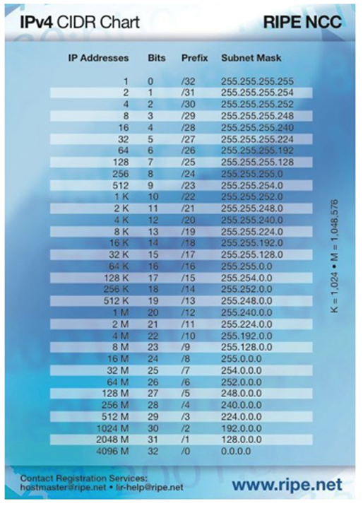
Here’s a picture of all possible subnet masks you can use in IPv4:

So you have a subnet and a bunch of addresses you can use...
... but not all of them can be used for hosts.
Three are reserved for:

The subnet network address (e.g. 152.78.70.0)
The subnet broadcast address (e.g. 152.78.70.255)
The address of the router, also called gateway (any other address within the subnet range, but conventionally either 152.78.70.1 or 152.78.70.254)

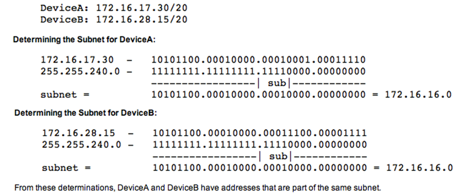
How do you determine a subnet (network) address?
Take the IP address and subnet mask (derived from the prefix length), and binary AND them to get the subnet network address.

How do you determine a subnet broadcast address?
Take the IP address and wildcard mask, that is the inverted binary subnet mask, and binary OR them to get the subnet broadcast address
Determining the broadcast address for a device with IP address 172.16.17.30 and subnet mask 255.255.240.0 (/20), which is the wildcard mask 0.0.15.255:

172.16.17.30	10101100.00010000.00010001.00011110
0.0.15.255	00000000.00000000.00001111.11111111
Broadcast =	10101100.00010000.00011111.11111111	= 172.16.31.255

ARP can also be used to find the Ethernet (MAC) address of the default router (gateway) of the network (if the destination IP is not in the same subnet).
This is why being able to use the subnet mask to determine the subnet address is important.

What happens if you screw up the subnet mask (e.g. if the network admin misconfigured the value on the DHCP server)?
If it’s too short (it is /23 when it should be /24)

Host may think a remote host is local, so it’ll use ARP locally
It won’t get a response

If it’s too long (it is /25 when it should be /24)

Host may think a local host is remote, so it’ll send it to the router
The router may end up redirecting the packet

Calculating subnets

Here is a concrete example of how to calculate subnets - you could find a question like this in the exam:
You have been tasked with assigning IPv4 address ranges to six subnets in a new building and specifying the routing tables. You have been allocated 152.78.64.0/22 to carry out this task. How would you allocate this block of addresses to best use the available space to cater for …? In your answer you should include the network address, the broadcast address and prefix length of each subnet!

A computing lab with 260 computers
First of all, let’s determine the subnet size we need. We want to find the smallest power of two that exceeds the host count by at least three. Why three? Because one is the network address, one is the broadcast address and one is reserved for the gateway (default router). Why the smallest? Because we do not want to waste any addresses by making our subnet too large.
In this case, it is 9 because 2^9 = 512 and 512 - 3 >= 260.
So for this subnet, we will need the last 9 bits for the hosts, thus the first 32 - 9 = 23 bits are used for the network and stay fixed (Why did I use 32? Well, the whole IP address has 32 bits). Our subnet will be a /23 subnet.
Next, determine the network address for this subnet. The network address is always the lowest address. Since this is the first subnet, we are going to start with 152.78.64.0, which is given in the question.
Finally, we need to determine the broadcast address. Our network address is 152.78.64.0 and our subnet mask is /23. The broadcast address is always the highest address. Therefore we need to copy the first 23 bits and leave them unchanged, and take the last 9 bits and set them to 1.
After you do this you will get 152.78.65.255, which is our broadcast address.
So all in all our subnet is 152.78.64.0/23 with the broadcast address 152.78.65.255

An electronics lab subnet with 200 computers
Again, we will determine the subnet size first. This time it is 8, because 2^8 = 256 and 256 - 3 >= 200. Therefore our subnet will be a 32 - 8 → /24 subnet
To determine the network address, take the broadcast address of the last subnet and add 1. Why 1? Because we don’t want to leave any gaps and thus waste addresses in our allocation. 152.78.65.255 + 1 → 152.78.66.0 (by doing this, we ensure that this subnet begins immediately after the last one ends) Attention: This only works if the current subnet is of the same size or smaller than the last one. Otherwise, you might need to leave a gap. You can check if you need to leave a gap by checking whether the network address is the lowest one in the range. If it isn’t, you must leave a gap and skip to the next possible network address.
To determine the broadcast address, take the first 24 bits of the network address and set the last 8 bits to 1. Luckily, the first 24 bits are exactly the first 3 groups. Now we get 152.78.66.255.
All in all, our subnet is 152.78.66.0/24 with the broadcast address 152.78.66.255.
An office subnet with 110 computers
Subnet size: 2^7 = 128, 128 - 3 >= 110 → /25
Network address: 152.78.66.255 + 1 → 152.78.67.0/25
Broadcast address: 152.78.67.127
Also, an alternative way to calculate the broadcast address if you already have the network address is to just add the subnet size - 1 to the network address. In this case the subnet size is 128 addresses, so we will add 127. Take 152.78.67.0 + 127 → 152.78.67.127 and you are done. Attention: this only works if you add to the network address, the other procedure works with every address within the network! This technique is especially helpful if the subnet size is 8 or smaller.

A server subnet with 60 servers
Subnet size: 2^6 = 64, 64 - 3 >= 60 → /26
Network address: 152.78.67.127 + 1 → 152.78.67.128/26
Broadcast address: 152.78.67.128 + 63 → 152.78.67.191

A DMZ subnet with 25 servers
Subnet size: 2^5 = 32, 32 - 3 >= 25 → /27
Network address: 152.78.67.191 + 1 → 152.78.67.192/27
Broadcast address: 152.78.67.192 + 31 → 152.78.67.223

An infrastructure subnet with 17 devices
Subnet size: 2^5 = 32, 32 - 3 >= 17 → /27
Network address: 152.78.67.223 + 1 → 152.78.67.224/27
Broadcast address: 152.78.67.224 + 31 → 152.78.67.255

We are done. As a last cross-check we can verify whether our allocation fits within the range we were initially given. Wait, you don’t need to scroll up, it was 152.78.64.0/22.
Let’s determine the broadcast address. Be careful, because it might be the case that the address given is not the network address (i.e. the lowest address) of this range, so you may not be able to just use the trick I previously used and add 1023 to this address!
To determine the network address, take the first 22 bits and leave them unchanged. Set the remaining 10 bits to 0. You will get 152.78.64.0, so as it turns out, the address given was indeed the network address (which is the lowest address).
To determine the broadcast address, either set the last 10 bits to 1 or just add 1023 to the network address. You will get 152.78.67.255, which is exactly the broadcast address of our last subnet.
So to conclude, our allocation fits perfectly in the range that we were initially given.

ICMP

ICMP (or Internet Control Message Protocol) is a supporting protocol for sending status messages between hosts instead of actual data.
If you ping a host, that’s ICMP.
ICMP can be used to send error messages or other operational information.
ICMP can also be used for routers to tell other routers about themselves to fill out their routing tables, called router advertisement.

IP routing protocols

When a host sends a packet, it will send it:

directly to the destination, if it’s on the same local subnet
to the router, if the destination is not on the local subnet

Hosts have no idea what goes on outside their subnet; they just send to the router and let that take care of the rest.
The router will participate in a site routing protocol, and the site routes to the Internet using a policy-rich routing protocol called Border Gateway Protocol (BGP).

To determine whether to deliver locally or forward to a router, a host maintains a small routing table, with a list of known networks and how to reach them (can be built from information learnt by DHCP or IPv6 RAs)
The table includes a local subnet in which the host resides, and a ‘default’ route to send a packet if the destination is not in the routing table (the ‘default’ route is usually to the router / default gateway)

But when a packet gets to the router, what do we do then?
The router needs to try to forward the packet to the destination’s router.
This is where we use routing protocols!

So, how do we solve this problem?

Static routing:

We configure the routes manually.
It works, but if the topology changes or network faults occur, we have problems

Dynamic routing:

We use routing protocols to establish a route on-the-fly, such as:

Routing Information Protocol (RIP) - distance vector algorithm
Open Shortest Path First (OSPF) - link state algorithm
IS-IS - link state algorithm

Aggregating prefixes

You’d think all routers would need to have access to all other routers on the Internet to communicate, right?
No need; aggregated prefixes exist!
Instead of routing to 152.78.70.0/24 exactly, you can route to 152.78.0.0/16, and through there the packet can find its way into the smaller subnets, like 152.78.240.0/20, 152.78.255.128/25, and any subnet with address 152.78.??.??/x where x is greater than 16.
Let’s look at an example:

Here, R1 serves 152.78.2.0/24 and R7 serves 152.78.64.0/23.
Instead of sending directly to R1, we can send our packet to the border router, which serves 152.78.0.0/16, which makes it an “umbrella” router for all addresses 152.78.0.0 to 152.78.255.255.

Interior routing protocols

Routing is all about routers maintaining routing tables and looking up destination addresses to know where to send off the packet to.
The routing table is, fundamentally, a table with destination IP prefixes and the interface or next hop to use.
So how do routers fill in their routing tables? Routing protocols! They allow routers to build or exchange routing information.

Distance Vector

With the distance-vector routing protocol, we determine the best route from one router to the next by distance, the distance being the number of routers (or hops) from the source to the destination.
It does this by only talking to the directly neighbouring routers in a site, and uses an algorithm such as the Bellman-Ford algorithm to get the shortest distance.
An application of this would be the Routing Information Protocol (RIP).

RIP is just an application of the distance-vector protocol, but with a few extra conditions.
Each router maintains a RIP routing table, storing:

Destination network
Cost (hop count); 0 if network is directly connected
Next hop to use for best path

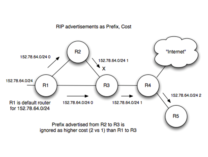
If a router receives an update with a lower cost path to a destination network, it updates its entry for that destination
If a router receives a higher cost path later for the same destination from the same neighbour, the higher value is used because topologies can change and the lower cost route might not be valid anymore

This is all great, but RIP isn’t perfect:

Updates are only sent every 30 seconds, so things take time. Plus, updates aren’t acknowledged (UDP) so there could be message loss
Metrics are simple hop count values. What if you wanted to weight certain links? Plus, the maximum value is 15. A value of 16 means unreachable.
Routers don’t have knowledge of network topology, so this can lead to the ‘count to infinity’ problem (basically, a loop)

Link state

With the link-state routing protocol, we talk to all routers and establish full knowledge of the site
Routers flood information messages describing their connected neighbours around the entire site
An application of this would be IS-IS (Intermediate System to Intermediate System) or OSPF (Open Shortest Path First).
The steps are as follows:

Discover neighbours
Determine cost metric to each neighbour
Construct link-state information packet
Flood this message to all site routers in the same area
Use messages to build topology, and then compute shortest paths for prefixes served by any given router

The cost is usually based on bandwidth/delay

The structure of a link state packet is as follows:

Source ID to uniquely identify the node
Sequence to allow receiver to determine if message is a new one to process and flood, or one to discard (sender increments sequence number with each message)
Age (decremented once per second, prevents old messages persisting in the network)

All messages are acknowledged to senders

Because we know the whole topology, we don’t need to use Bellman-Ford or anything. We can just use Dijkstra’s, which is faster.

Exterior routing protocols

Autonomous system (AS): a network or a collection of networks that are all managed and supervised by a single entity or organisation, typically an ISP (Internet Service Provider).
An interior routing protocol is for exchanging routing information between gateways (routers) within an autonomous system.
In contrast, exterior routing protocols are for exchanging routing information between autonomous systems.

The de facto exterior routing protocol is Border Gateway Protocol (BGP).
In BGP, each ISP has a unique AS Number (ASN), assigned by RIRs (Regional Internet Registry) -they’re 32 bits long
It’s like distance-vector, but BGP includes many improvements and also incorporates the AS path associated with using a given route, the costs of the paths and many other richer attributes.

In BGP:

BGP neighbours, called BGP peers, are identified and create TCP sessions over port 179
They send their whole routing tables to each other, and send incremental updates when something changes
Then, the routers advertise routes they know to their neighbours, containing network prefix, prefix length, AS path, next hop etc.
Neighbours can then use their knowledge of ASNs to choose whether to use that route or not

Here is an example:

F needs to get to D, but how? To get to D, F will have to go through one of its neighbours. But which neighbour should F choose?
To choose, F asks all its neighbours how they would get to D. F will then pick the neighbour with the shortest distance.
F will obviously not pick I or E, because their paths contain F itself.
F will likely pick either B or G, making the path from F to D either FBCD or FGCD.

Transport layer

The transport layer handles how the information is going to be transported from the source to the destination.
There are two protocols that the transport layer can use: UDP and TCP

UDP

User Datagram Protocol (or UDP) is a connectionless protocol on a ‘fire and forget’ basis.
Packets are sent to their destination with no acknowledgements. They just sort of throw packets towards the destination and hope for the best.

The properties of UDP are:

Connectionless:

No need to set up a connection with the recipient

Application layer has to retransmit, if required:

If the recipient doesn’t get the data, the application layer is responsible for resending

UDP applications use a constant bit rate:

No need to control the bit rate as the packets all come in at once anyway
The application should adapt if necessary

Low overhead:

No connection management is used, so we use less bandwidth

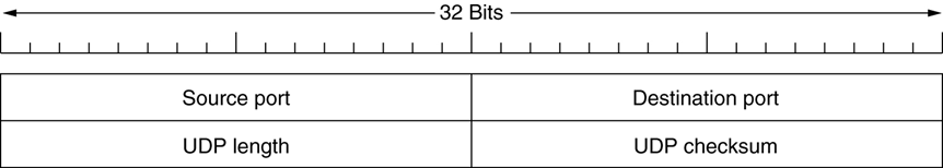
The UDP header is simpler than TCP’s header
The checksum is optional

If buffers are full, packets may be dropped. The application can detect this and tell the server.

TCP

Transmission Control Protocol (or TCP) is a connection oriented protocol.
It includes acknowledgements and retransmissions.
TCP provides performance and reliability on an otherwise unreliable IP service, at the expense of an overhead.

The properties of TCP are:

Provides connection management:

A connection is established and managed

Provides flow control:

Slows down / speeds up when needed

Uses that capacity but tries also to avoid congestion:

Backs off when there’s packet loss (indicator of congestion)

Retransmission:

Sends segments again if they were unacknowledged

Receiver reassembles segments in the correct order

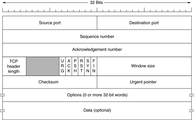
TCP headers are padded so that they’re a multiple of 32 bits.
Seq and Ack numbers used to track sequential packets, with SYN bit:

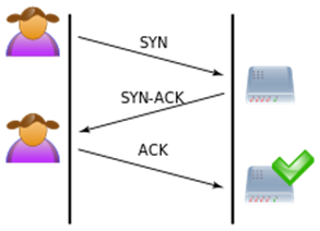
TCP connection establishment uses a three-way handshake of:

SYN: “Can I talk to you please?”
SYN-ACK: “You may talk to me.”
ACK: “We are now talking.”

Each side uses a sequence number, so both parties have a common understanding of the position in the data stream

The sender must detect lost packets either:

by retransmission timeout:

Estimate when ACK is expected

by cumulative acknowledgement (DupAcks):

A type of acknowledgement that acknowledges all past data chunks

TCP uses a sliding window protocol, like go-back-N or selective-repeat back in the link layer, to perform flow control.
Basically, the window is the same size as the recipient’s buffer space. That way, the sender can’t send any more than the recipient can handle.
Once the recipient says that it can handle more, the window is slid and further packets will be sent.

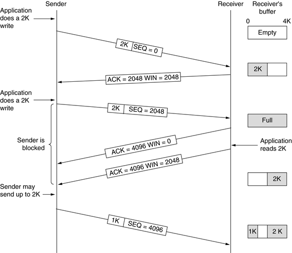
The sender sends a segment with a sequence number and starts a timer.
The receiver replies with an acknowledgment number showing the next sequence number it expects and its available buffer/window size.
If the receiver doesn’t send anything by the time the timer goes off, the sender resends.
If the receiver says the window size is 0, the sender may send a 1-byte probe to ask for the window size again.

Here is an example, with dialogue to show you what’s going on:

LEFT: “This is packet 0 (#1), it’s 2K in size”
RIGHT: “Nice; I want packet 2048 (#2), and I have 2048 bytes of space left”
LEFT: “Here’s packet 2048 (#2), it’s 2K in size”
RIGHT: “Great; I would want packet 4096 (#3) now, but I’m full (I have 0 bytes of space)”
RIGHT: “OK, I want packet 4096 (#3) now, and I have 2048 bytes of space”
LEFT: “Alright, here’s packet 4096 (#3), it’s 1K in size”

If the connection started to get congested, how does TCP control this?
TCP actually has two windows: a “recipient buffer” window and a congestion window.
The recipient buffer window is defined just above; it’s how much the receiver can take in before it gets full.
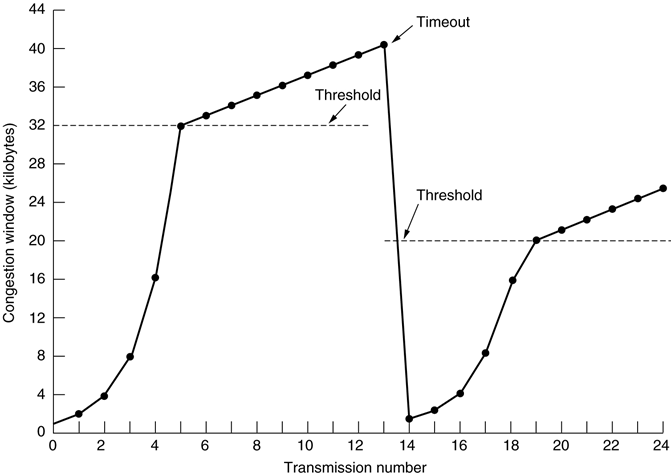
The congestion window does its best to prevent congestion in the connection (too much data flying through means more packet loss)
A congestion window starts off small, and grows if everything is going alright. It resets if there is a timeout.
The window size doubles each time, until a threshold is reached, at which point it’ll increase linearly, called Congestion Avoidance.
After a timeout, the threshold decreases a bit.
So which window do we use; the recipient buffer window or the congestion window?
We use whichever one is smallest.
Here is a graph showing the size of the window changing with each transmission:

TCP or UDP?

Streaming services and voice over IP use UDP because it’s immediate and has limited buffering.
Web services like HTTP and SMTP use TCP because having a structured connection is more important.
DNS uses UDP because the overhead for TCP would be too much for processing 100 to 1000 requests per second.

Here are the differences between TCP and UDP:

	TCP	UDP
Connection	Connection oriented	Connectionless: “fire and forget”
Reliability	Handles ACK & retransmissions	Application needs to handle ACK & retransmissions if needed
Data Order	Guaranteed that it arrives and in the correct order	No guarantee that data is received in the order sent
Header	20-bytes minimum	8-bytes
Good for	Applications that need high reliability	Applications that need fast and efficient transmission
Example protocols	HTTP(S), FTP, SMTP, Telnet, SSH	DHCP, TFTP, SNMP, RIP, RTP, COAP

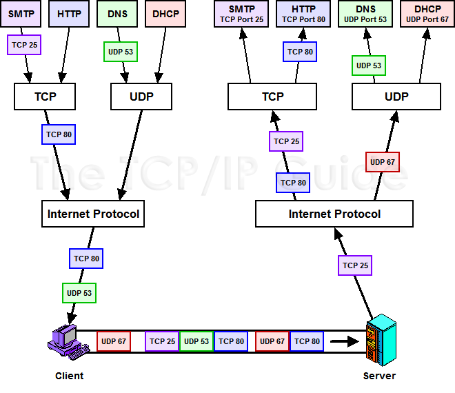
Here is a graphic showing the layers and what protocols they use:

Sockets

A socket is created when a sender and a receiver act as communication endpoints.
A socket has an IP address and a port number, for example 152.78.70.1 port 80
The socket and bind protocol uniquely identify the application’s subsequent data transmission.
When multiple clients talk to one server, there is usually one thread per client endpoint.
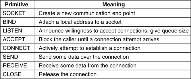
There is a sockets API, called the Berkeley sockets API. Servers mainly use SOCKET and BIND, whereas clients tend to use SOCKET and CONNECT:

DNS

First of all, what is a DNS?
The Domain Name System (or DNS) is a naming system for pairing up domain names to IP addresses.
For example, when you search up “google.com”, you’re actually talking to an IP, such as “216.58.213.110”, and the DNS translates “google.com” to that IP for you.

DNS names are delegated through the Top Level Domain (TLD) registrars
For example, with soton.ac.uk:

first the “.uk” bit is delegated by Nominet
then the “.ac.uk” bit is through Jisc
then finally, the whole thing “.soton.ac.uk” comes down to the University of Southampton

It allows sites and organisations to maintain authority over their registered domains.

The most common DNS lookup is host name to IP.
The DNS returns an A record for IPv4 or AAAA record for IPv6 when queried for a specific host/domain name.
This means clients need to know the IP addresses of local DNS servers (resolvers) so they can actually send the queries.

A DNS resolver is a server that acts as a DNS server that resolves queries and sends an answer back.
Client hosts are configured to use one or more local DNS resolvers. They’re usually provided via DHCP.
Clients can use APIs to do DNS lookups. You can even do it via a CLI tool.

Packets sent to DNS resolvers are usually UDP packets, but they can use TCP.
They use UDP because it’s connectionless and quick.
The results of queries can be cached.

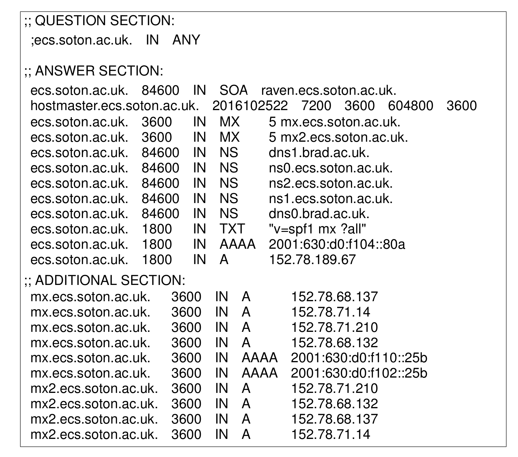
Here is a list of DNS record types:

Campuses will run their own DNS servers, so they can:

act as resolvers for internally sourced DNS queries
act as servers for external queries against internal names

Some DNS infrastructures also may provide a ‘split DNS’ view, which is where separate DNS servers are provided for internal and external networks as a means of security and privacy management.

If DNS servers are local, then how does a client talk to a server from across the world?
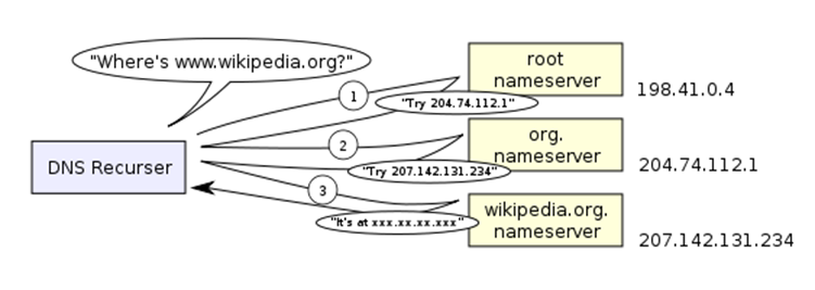
We leverage the hierarchical delegation structure! What? That doesn’t make sense?
Basically, we have a set of “root” DNS servers that can point us to other DNS servers that know about different URL suffixes.

For example, if we were looking for “www.google.co.uk”, the root DNS could point us to another DNS server and say “go to them, they know all about URLs ending in uk”
Then that DNS server could point us to another DNS server and say “go to them, they know all about URLs ending in co.uk”
... and so on until we reach a DNS that knows the IP address for www.google.co.uk.
Mapping one DNS to another DNS is known as DNS glue.
So in other words, to get your IP from your host name, your browser goes on one big adventure, going from DNS to DNS, looking for the IP.

This can also be cached, so we don’t hit DNS servers heavily.

DNS resolvers are critical to Internet infrastructure.
Because of this, people like to attack them.
Therefore, we need to make them resilient and strong.

Root servers are the ‘anchor’ for recursive DNS’.
If someone managed to shut down all the root servers, they could shut down the Internet.
There are 13 highly available clusters of root servers. There are about 1000 servers in total used in these clusters, and a server is picked in a cluster via anycast.

This makes DNS servers more distributed and allows clients to use the most local server, improving performance.
It also helps spread the load, and mitigate DoS attacks.

IP anycast is where the same IP is configured in many locations, and your network picks the closest one to connect to.
This is especially applied to DNS servers, as picking the closest DNS server means you get better performance.
It also means you don’t have to reconfigure your network when you’re in a different place; because of anycast, your network just picks the closest DNS server anyway.

Fast flux DNS is a technique where the association between an IP address and a domain name is changed very frequently.
This is used in some peer-to-peer systems, but it can also be used by botnets (the bad guys) to avoid detection and make takedown harder (so they don’t get caught by the good guys)

Public DNS servers are open public servers. They also answer queries for domains, recursively. An example is the Google public DNS server.
Why use them?

Speed improvements
Reliability
Parental controls
Phishing protection
Security
Access geoblocked content
Bypass web censorship

However, you don’t know who’s logging your queries (and with a company like Google, can you really trust them?)

Application layer

The application layer provides higher level services.
In the TCP/IP layer, it’s just called “Application”, but in the OSI Model layers, the application layer is split up into “Application”, “Presentation” and “Session”.

Telnet

Telnet: Simple unencrypted terminal emulation protocol
In other words, it provides a bidirectional text-based communication service using your terminal, like a Unix / DOS chatroom!
It was big in the 90’s, but nobody really uses it anymore because

It’s old and computer normies non-techies don’t like using terminals
It doesn’t even have security, it’s unencrypted

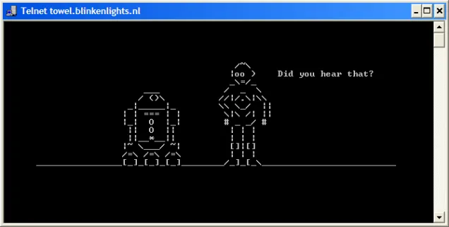
Today, it’s mainly used as a plot device in films (like Die Hard 4) and watching the original Star Wars in ASCII (the server is towel.blinkenlights.nl) .

Email

There are two main protocols for emailing: SMTP and IMAP.

SMTP

SMTP (Simple Mail Transfer Protocol): a protocol used to send emails.
It uses TCP to connect to a mail server and uses the commands MAIL, RCPT and DATA.
Authentication is an extension; you don’t need it, but you should have it by now. Original emails didn’t have it.
You can use SMTP quite easily in modern languages, like Python and PHP.

How does SMTP work? Well, if you’ve been reading my notes, you know I prefer to go in detail about stuff like this (within reason).

If this illustration isn’t enough, here’s some dialogue, where Alice is the sender and Bob is the receiver:

Alice: “Hey, do you want to start a TCP connection?”
Bob: “Yes. Let’s talk in TCP.” (220 message)
Alice: “Alright, let’s begin. Hello! Tell me what you can do.” (EHLO extended hello message)
Bob: “OK. Here’s what I can do: (a list of things Bob can do)” (250 message with list of supported SMTP extensions)
Alice and Bob start performing mail transactions (you don’t need to know these)
Alice: “I’m done with you. Let’s stop talking.”
Bob: “OK. Goodbye.” Bob stops listening to Alice (221 message, Bob closes transmission channel)
Alice receives Bob’s goodbye and also stops listening to Bob.

IMAP

IMAP (Internet Message Access Protocol): a protocol used to retrieve emails.
It was designed in 1986 and listens on port 142 (993 for the secure version)
It keeps a TCP connection open to send requests or receive notifications.

HTTP

HTTP (HyperText Transfer Protocol): a text-based protocol that uses TCP and uses port 80.
There are two steps to using HTTP:

Send a request (e.g. GET /something/page.html HTTP/1.1)
Receive a response message (e.g. HTTP/1.1 200 OK)

A typical response might contain things such as:

Version of HTTP
HTTP status code
Date
Content type (text, html, xml etc.)
Server type

The main types of HTTP requests are:

GET - simply retrieve data
HEAD - like GET but no data is sent back
POST - send data to server, usually to create records
PUT - send data to server, usually to edit existing records
DELETE - send data to server, usually to delete a record

You can tell the variety of a status code by the left-most digit:

1xx -> Information
2xx -> Success (e.g. 200 ok)
3xx -> Redirection (e.g. 301 moved)
4xx -> Client error (e.g. 403 forbidden, 404 not found)
5xx -> Server error (e.g. 500 internal error)

You can send HTTP requests using the wget or curl commands in Linux.

HTTP/2

The first major revision to HTTP, published in 2015
The header is now compressed as binary using HPACK, a header compression algorithm. However, now, the whole packet is binary, not just the header.
It also has Server Push, which means resources are sent to the client before they even ask for them. No, it doesn’t use King Crimson and erases time, instead it goes like this:

Let’s say you requested index.html, and that page uses styles.css and script.js. Normally, you’d request for index.html, receive that, find out you need styles.css and script.js, and do separate requests for those assets, too.
With Server Push in HTTP/2, the server already knows that you’ll need styles.css and script.js, so it prepares those responses in advance before your browser even has the chance to parse index.html.

It can also multiplex multiple requests over a single TCP connection.

QUIC

QUIC (Quick UDP Internet Connections): A UDP protocol to make the web faster, and possibly replace TCP.
It’s pushed by Google, and it still establishes some “state”/sessions and encryption.
It’s experimental, which is why you’ve probably not heard of it.
HTTP/3 will be based on QUIC instead of TCP.

CoAP

CoAP (Constrained Application Protocol): provides HTTP-like protocol for simple devices
It has a minimal overhead, perfect for small devices.
Binary encoding for GET / PUT / etc.
It has a simple discovery mechanism and a simple subscribe method
It’s used in things like Ikea smart lighting.

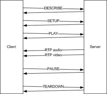
RTSP

RTSP (Real Time Streaming Protocol): a protocol used for streaming video / audio
It’s used by YouTube and Flash players (R.I.P.).
Video frames are packetized so that losses do not corrupt the whole stream.
It has a URL scheme with arguments, similar to HTTP GET.
Real-time transport protocol (RTP) delivers the media (typically with UDP).

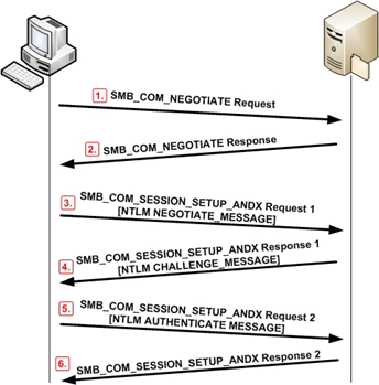
SMB

SMB (Server Message Block): a file-sharing protocol from Microsoft that can use either TCP with port 445 or UDP.
It provides authentication, file locking etc.
It’s provided in Samba within Linux.

NFS

NFS (Network File System): a file-sharing protocol mainly used in Unix / Linux.
It’s common between servers and can cope with very large files and file numbers.

P2P

P2P (Peer-to-peer): instead of using a server-client model, every device has the same priority and shares data with each other.
It distributes the content efficiently across everyone, instead of having one master device rule all.
BitTorrent uses this for files (as you probably know).

IPv6

Why do we need IPv6?

We’re running out of IPv4 addresses!
The organisations handing out IP addresses (called RIRs) have no unallocated address blocks.

It started off with alpha support in 1996, but drafts for the IPv6 standard was established in 1998.
In the bizarre summer of 1999, IPng Tunnelbroker started, which “tunnelled” v4 to v6.
They started putting them in servers at 2004, but major PC operating systems didn’t start supporting them until 2011.
Now, people are starting to use it more, for instance in 2016 Sky has 80% IPv6 coverage.
It became an internet standard in July 2017.

IPv6 Features

So what can v6 do?
It has a 128-bit address, as opposed to the 32-bit v4 address, so there’s IPv6 addresses.
If we gave each grain of sand on Earth a global address, we’d only take up 0.000000000000000002%, or of the total number of addresses we have.
To put it in perspective further, if we had a copy of Earth for every grain of sand that exists on this Earth, and we gave global addresses to all the grains of sand on every copy of Earth, we’d still have addresses left over! Basically, that’s a lot of addresses.

IPv6 addresses are usually written in colon-separated hex format, to keep it shorter.
Leading 0’s are also omitted, and a single set of repeated 0 blocks can be replaced with “::”.

e.g. address 2001:0630:00d0:f102:0000:0000:0000:0022
can be shortened to 2001:630:d0:f102:0:0:0:22
which can be shortened to 2001:630:d0:f102::22

Remember that you can only do this once, or else there will be confusion over where the zeros are! Source

Some other features include:

Subnets are represented in CIDR notation (like v4, e.g. 2001:630:d0:f102::/64)
Not as easy to remember as v4 because it’s longer, but you shouldn’t care
Multicast is an inherent part of v6, and used in subnets instead of broadcast
v4 and v6 can co-exist in dual-stack deployments

Just like how v4 had preset addresses, v6 has address scopes dedicated to certain tasks:

::1/128 - loopback
::/128 - unspecified (equivalent to 0.0.0.0)
fe80::/10 - Link-local address (used only on local link)
fc00::/7 - Unique Local Address (ULA, used within a site)
2000::/3 - Global Unicast
ff00::/8 - Multicast

Hosts usually have multiple v6 addresses!

There are conventions, too:

/127 can be used for inter-router links
Smallest subnet is a /64 (which still allows 18 quintillion addresses)
Home / small business users should be given a /56
A “site” is usually given /48
Minimum v6 allocation from RIR is /32

Any subnet larger than /64 can be used

We know that v4 addresses are running out, but are there any technical benefits to v6?

No more NAT
More “plug-and-play” than v4 (require less setting up as Stateless auto configuration (SLAAC) works)
Streamlined header, so more efficient routing and packet processing
Fragmentation occurs at sender, so less strain on routers

Why use v6?

If v4 works for now, why swap to v6 early?

You should get familiar with v6 before it becomes mandatory
You can secure v6 and still use v4
Support for new applications
Enables innovation / teaching / research

To be fair, those last two are only for companies.

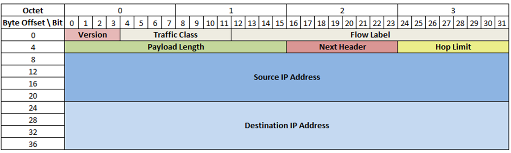
IPv6 headers

IPv6 headers are a fixed 40 bytes, which is bigger than IPv4, but simpler.
It uses extension headers rather than options, and has 8 fields:

Version: represents the version of the Internet Protocol i.e. 0110
Source Address: the address of the originator of the packet
Destination Address: the address of the recipient of the packet
Traffic class: indicates class/priority of the packet
Flow label: a “hint” for routers that keeps packets on the same path
Payload length: size of the payload + extension headers
Next header: indicates the type of the next header
Hop limit: equivalent to the “time to live” field from v4

Extension headers carry optional Internet Layer information, and sits after the v6 header but before the transport layer header in the packet.

It’s equivalent to the options field in v4
Fragmentation is an extension header
Extension headers can be daisy chained, but must be in order
Each extension header has a “next header” field, hence the daisy chaining

Each extension header is a multiple of 8 bytes

IPv6 with routers and privacy

The way v6 handles neighbour discovery replaces ARP and ICMP Router Discovery.
There are five ICMPv6 packet types:

Router solicitation: host requests router information
Router advertisement: tells other routers about itself
Neighbour solicitation: equivalent to ARP “who has __”
Neighbour advertisement: equivalent to ARP reply
Redirect: router informing host of a better first-hop (in other words, a router correcting a host of a more efficient path)

When a host sees or solicits a Router Advertisement (RA):

The RA message carries the v6 network prefix (/64) to use
The RA source address implies the default router address
DNS server information can be in the RA

Prefix information is sent by multicast:

Periodically (usually every 600 seconds)
On request (in response to a Router Solicitation)

IPv6 can also automatically configure basic network settings without a DHCPv6 server, using something called StateLess Address AutoConfiguration (SLAAC).
A host using SLAAC builds it’s address from:

A 64-bit prefix from a Router Advertisement
A 64-bit host part generated from the MAC address

It’s a security issue to embed your MAC address in your global address, because the host part stays the same across networks, meaning it’s easier for people to track you.
A privacy extension of RFC 2941 adds a random 64-bit host part, used for outgoing connections, to mitigate this issue.

There’s an alternate method too in RFC 7217 that does not use a MAC address, and it mitigates many of the security / privacy issues of before.

Deploying IPv6

The Internet is mostly v4. How do we get all the benefits of v6?
One approach is: “why not both?”. It’s called “dual stack”.
We might also have v4-only systems or v6-only systems that need to talk to each other.

A dual stack system runs both v4 and v6 on the same equipment.
You may need to rewrite/update applications and pick when to use v6 or v4 (typically, it’s use v6 if available)
You still require a v4 address space, because you use v4, and you need to secure both protocols (e.g. firewall).

How do you translate from v4 to v6 and vice versa?
You could:

Rewrite the header information
Use Application Layer Gateways (ALGs)
NAT64: a Nintendo 64 game using NAT to convert single IPv4 address to IPv6 network
DNS64: “fabricates” AAAA record for non-IPv6 sites that points to an IPv6/IPv4 translator

There’s also a variety of tunneling technologies to use:

6in4 - encapsulates v6 packets in v4 packets
Teredo - encapsulates v6 into UDP v4
DS-Lite (no, not the console) - encapsulates v4 packets in v6 packets
VPNs work too

What’s the best? Like Totally Spies, there is no best; some are suited to certain scenarios.
We’re still going to use v4 for a long time, but the focus at the moment is dual-stack. v6-only is growing, though.

Everyone’s using v6 now! Youtube, Dropbox, LinkedIn, Wikipedia, major ISPs...
Home routers lack v6 support because people in general (normies) don’t want to learn something new, and network administrators lack the desire to understand v6.

IPv6 security

IPSEC encryption is baked into v6.
There’s tonnes of addresses (as you know), so scanning is less feasible.
Transition mechanisms (like tunneling and Teredo) can bypass network security mechanisms.
v6 implementations still have flaws that are undiscovered (e.g. Windows is susceptible to Router Advertisement flooding)

v6 hosts can pick their own address.
To track which devices are used where, we can poll switches and routers for MAC table and ARP table information.

Other IPv6 stuff

Don’t be an uninformed IPv6 normie! Know your stuff with this FAQ:

Q: We don’t need IPv6, with CGNAT and address recovery, we have a lot more addresses.
A: Those can only get you so far until you come crawling back to IPv6.
Q: IPv6 replaces IPv4
A: Wrong. They will co-exist for years to come.
Q: IPv6 is more complicated than IPv4
A: The concepts are similar or simpler. You’re just lazy.
Q: IPv6 is less secure because there’s no NAT
A: NAT isn’t a security mechanism and v6 has firewalling/ACLs.
Q: IPv6 probably won’t be in the exam, so I won’t revise it
A: Fool! It’s Sod’s Law that the one thing you don’t revise on will be on the exam. I know it’s boring, but please read all the sections.

As long as you know these answers, you can now become “that guy” by preaching to everyone about how IPv6 is the best thing ever and that you’re better than everyone still using IPv4!

So, summary pls?
IPv6 good, IPv4 bad

Network security

Security is very important, as you know.
You can never be 100% secure!
The human element is often the weakest link in a system, hence why things like phishing is so harmful.
Anyone can be an attacker, and they can have any motive, so stay sharp and read this section to pass the exam be more aware of cyber attacks!

DNS Security

DNS can be exploited to break something!
A DNS amplification attack is an attack where:

The attacker sends tons of messages to a DNS with the victim’s source IP
The DNS spams the victim with DNS response messages
The victim is overloaded with DNS messages and dies (not really, but you get the picture)

So how do we trust DNS responses?
It’s not signed or encrypted, and messages can be spoofed, so no, we can’t trust DNS responses.
There was even a campaign called DNSpionage which used this.

OK, so DNS is insecure, but what information could it possibly leak?
Well, your connection to a server may be encrypted, so what you’re doing is safe. But since DNS is insecure, where you’re doing it isn’t safe.
This means third parties know where you’re doing stuff, and that’s usually all they need to know to get your usage patterns.

So, that’s it? Privacy is dead and we’re all going to die?
Not quite: DNSSEC addresses DNS insecurity and was developed 10 years ago, and is still being worked on to this day.
It allows responses to be signed, but that makes them bigger and more complex to manage. Still, it’s worth it.
Lots of people deploy it (like Jisc for .ac.uk and Nominet for .uk), but some haven’t yet (like iSolutions for .soton.ac.uk).
There’s other things too, like blocking non-local look-ups, or ignoring certain kinds of requests.

Firewalls

NAT is NOT a security mechanism!!! >:0 (I mean, I don’t remember anyone saying it was, but oh well)

A firewall is a network device that sits at the edge of a network and operates at the Network layer.
It acts as a packet filter, and blocks packets that do not fit a set of rules.
Stateless firewalls, or firewalls that work simply by testing predicates on packets, are limited (e.g. to allow all packets on port 80 would mean an attacker can attack on that port).

Sod that; in this day and age, you want a stateful firewall!
These firewalls keep track of connections, and map packets to connections.
There are rules for related and established packets, e.g. allow outbound port 80 packets but disallow incoming port 80 packets unless it’s in relation to an existing connection, which makes sense; a server doesn’t just randomly give you a web page!
A common set of rules for home networks is:

Deny all inbound rules unless related / established
Allow all outbound

You can have even more powerful firewalls that act on the application layer.
These firewalls actually snoop around your packets, checking if they look like what they’re supposed to.
For example, look at these two packets:

Packet #1 on port 80

Packet #2 on port 80

<!DOCTYPE html>

<html>

<head>

<title>JoJo homepage</title>

</head>

<body>

<h1>Joseph Joestar</h1>

<p>maybe josuke too</p>

</body>

</html>

<!DOCTYPE html>

// i’m a real packet i promise

remove_folder(system32)

Packet #1 looks like an actual HTML document, whereas packet #2 looks shifty and suspicious. An application layer firewall might be able to spot the difference.
However, this won’t work in all cases, especially when packets are encrypted, as SSH might look like HTTP.

At home, everything is packaged into one platform:

a router
DNS resolver
DHCP server
NAT implementation
network switch & wireless access point

At workplaces, you might have a firewall device on its own, or embedded in the router.

Intrusion Detection Systems

Someone may get into your network, or an actual user might do something stupid in your network.
How do you prevent this? Use NIDS (Network Intrusion Detection System)!
NIDS sniffs around in your network, looking for suspicious activity.
The detection may be signature based, or anomaly-based.
Some NIDS implementations might only be able to notify you, but some may be able to take action and prevent intrusion.

Port / Physical Security

If someone physically breaches a network, that’s a lot harder to protect against.
Fortunately, we have NAC (Network Access Control) mechanisms!

The simplest of which is to filter MAC addresses. However, it’s easy to circumvent and it has an administration overhead.

A better solution is 802.1x (creative name).
It uses Extensible Authentication Protocol (EAP) to authenticate clients.
It has three parties:

A supplicant (client)
An Authenticator (switch or access point)
An Authentication Server (e.g. LDAP using RADIUS)

It blocks the client until they authenticate themselves.
NACs can also have other features, like anti-virus

However, NAC doesn’t stop parties from sniffing traffic. Therefore, we need IPSEC (IP Security), which is encryption at the Network Layer.

There’s also VPNs (Virtual Private Network), that simulates a direct connection between devices.
It allows you to use internal services from the outside, and uses encryption.
There are two kinds:

Site-to-Site VPN: connects two different networks together, e.g. a branch office to head office
Remote-access VPN: where individual clients connect to a VPN server e.g. Globalprotect

These notes are brought to you by ExpressVPN!
Basically, if you didn’t know, a VPN is a service that encrypts your Internet data and gives you additional security!
It also works on phones and other devices!
You open the program, single tap, and it’s on!
I use ExpressVPN because privacy is important, keeps my information anonymous and safe from third parties.
Also, it has a 30-day money back guarantee and 30% off the first month when you use the code “NOTESNETWORK”.
Take back your Internet privacy today by clicking on the link: expressvpn.com/notesnetwork
And now, on with the notes!

WARNING: It’s a joke

DDoS

A DDoS (Distributed Denial of Service attack), or any DoS attack, is an attack that targets a system and puts them out of service to cause disruptions.
This can be done by consuming:

Network bandwidth
CPU cycles
Server state capacity
Other system resources

DoS attacks aren’t the focus; they’re usually used to distract others from the real threat, like:

Deploying malware
Stealing data

Single source attacks (DoS) are effective, but multiple source attacks (DDoS) can be more effective, as it deprives the target of more bandwidth, and it’s harder to stop as there’s lots of sources.

One example of a DDoS attack is the TCP SYN flood.
How it works is:

Attacker connects with target
Attacker sends “SYN”
Target sends “SYN ACK”, and is now expecting an ACK back
Attacker never sends ACK back

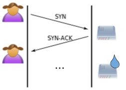
Normally, that wouldn’t be so bad for one client, but what if thousands of attackers did that at the same time?
It consumes state on the server and it doesn’t take much bandwidth to do; just lots of systems.

There are programs that can be used to perform a DDoS attack, like:

Low Orbit Ion Cannon (LOIC)
High Orbit Ion Cannon (HOIC)

There’s also a unique kind of DDoS called SlowLORIS, and is explained in detail here.

There’s also IPv6 RA flood, where you flood a target with IPv6 RA multicasts.
It makes targets join dud networks.
It’s mainly a problem with Windows, Mac OS and Linux aren’t really affected as much.

What are we going to do to prevent this?
There’s no clear way to prevent this, but there’s ways to mitigate it:

Anycast/content delivery networks: spread the load across lots of networks/systems
Responsive network team: block attacks as they occur and redistribute services across different connections
Good relationships with upstream providers: get them to help blocking attack traffic

DDoS is easy to attack with, but hard to defend against.

Wi-Fi (In)Security

Obviously, wireless networks are less secure than wired ones.
All clients have access to all traffic in a wireless network.
It’s clear that wireless networks require some kind of encryption.

One of the old wireless encryption methods is WEP (Wired Equivalent Privacy).
It uses a 40-bit or 104-bit key and 24-bit IV, and uses the RC4 stream cypher
It was proved insecure in the early 2000’s, so don’t use it anymore!
The FBI proved that WEP is crackable in 3 minutes.

So they made a better one: WPA and WPA/2.
WPA (WiFi Protected Access I) is more of a fix for WEP and used Temporal Key Integrity Protocol (TKIP)
WPA/2 (WiFi Protected Access II) is more complex than its predecessor and more secure, and uses a 128-bit AES (encryption standard).
WPA-Personal: uses pre-shared keys
WPA-Enterprise: uses 802.1x authentication (for that extra pinch of security)

WPA are not without their weaknesses though!

If you have a crap password, like “password” (who even uses that anymore) then you’re far more likely to get hacked, even using WPA.
If the generation of keys are weak, they can be “guessed” from the SSID e.g. old BT routers could have their keys guessed from a spreadsheet

Distributed Systems Implementations (Tim)

Distributed Systems Models

Physical models

There are really only 4 physical models:

Early 80’s: up to 100 nodes connected by LAN
Internet-scale (90’s): large nodes connected by Internet; nodes are static, not embedded and autonomous
Contemporary: hundreds of nodes, and nodes can change location. Can be embedded
Emerging: systems of systems

Architectural models

Types of communication paradigms:

Inter-process communication: low-level communication e.g. Java sockets
Remote invocation: two-way communication, sending and receiving
Indirect communication: one-to-many communication using groups, message queues, distributed shared memory systems etc.

Two main architectural models:

Client-server architecture: there’s one central “server” node, and lots of other “client” nodes that query a server with resources. Servers can also be used as clients.
Peer-to-peer architecture: all processes share similar roles, and data is distributed amongst peers. Used in software like Gnutella or BitTorrent.

Mapping entities to infrastructure

It’s not good enough to just have a cool network with lots of techy features.
Your system must be fit for purpose and be mapped to the infrastructure it manages.
For example, a logistics network could be mapped to road, rail, etc. infrastructure
How do we tailor our networks to fit into a mapping to infrastructure?
There are three strategies we can apply:

Use of multiple servers - several servers implement a service and distribute resources and services to increase performance
Proxies and caches - make web proxies store often used data to make it more quickly accessible
Mobile code - send code to the recipient, so they can run the code locally, which improves performance (but can also be a security threat)

Architectural patterns

There are several architectural patterns that networks can follow:

Layering
A vertical organisation of services into layers, with each service making use of the service below it (similar to OSI model or TCP/IP model)

Two-tier and three-tier architectures
Splits the system into different logic categories
For two-tier it’s view and modelcontroller

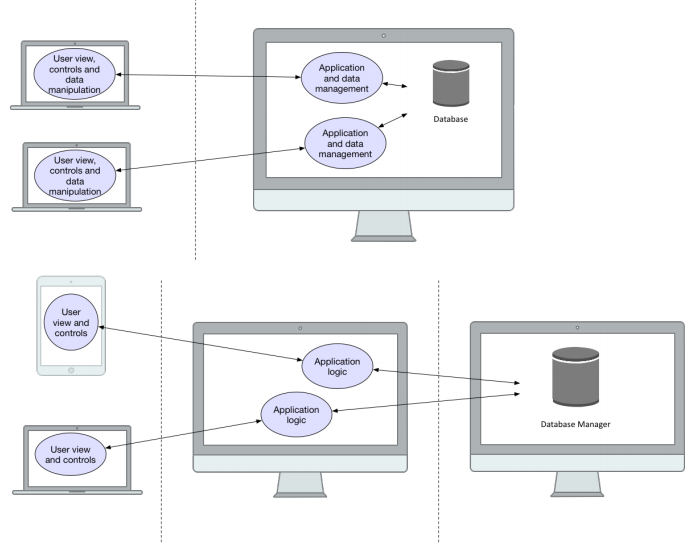
For three-tier it’s view, controller and model

Thin clients
Moves complexity away from the end-user and do all the hard computational stuff on the server.
Popular with Software-as-a-service (SAAS) in cloud computing
The point is that the client only has a handful of features (mainly a UI hooked up to some web requests) and the server does all the work
The opposite is called a thick client

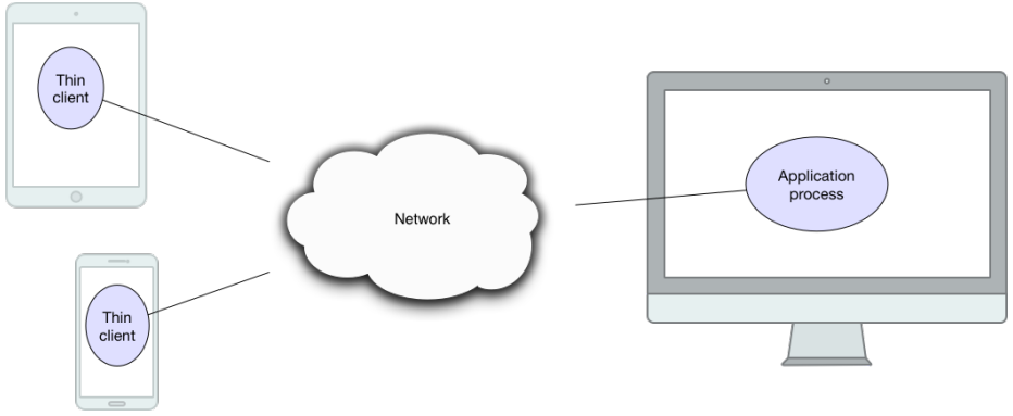
Proxies
Web proxies offer the same interface as the server they’re trying to mirror
Supports location transparency when doing RMI (remote method invocation)

Fundamental models: Interaction, Failure and Security

The three fundamental models include:

Interaction
Models how the participants interact with each other
There are two flavours:

Synchronous: we specify bounds about things like:

the time to execute each process step
the time to transmit a message over a channel
the drift of the local clock from real time

Asynchronous: we don’t care about stuff like that; messages can happen as and when

Often, distributed systems are asynchronous, which are harder to work with than synchronous because they need to handle actions in any order.
However, some problems can only be solved in synchrony (e.g. multimedia data stream)

Failure
Describes the types of failures that can happen, and what we can do to mitigate them
We categorise the types of failures:

Omission - failed to perform the action
Arbitrary (Byzantine) - performed the wrong action / lies
Timing - performed at the wrong time (only in synchronous systems)

We can mask failures either by:

Hiding - do something to rectify the failure (think of it like a try-catch)
Conversion - convert the failure to another kind of failure, so we can handle it (e.g. a corrupted message would initially be captured as an arbitrary failure, but we can convert it to omission once we realise it’s corrupted)

To ensure reliable one-to-one communication, you need:

Validity - every message is eventually delivered
Integrity - received message is identical to the one sent, and every message is only sent once

Security
Ensures security in both processes and communication
To ensure security, we need to model threats, more specifically a “man - in - the - mirror middle”
There are threats to both processes and communication:

Threats to processes: how can you trust the source of the message? An attacker can use a false identity when sending a request to the server (like a DNS amplification attack). You can’t tell.
Threats to communication channel: attackers can copy, alter or inject messages

But by using secure channels, we can kill two birds with one stone and patch these problems!

A secure channel uses existing encryption and authentication technologies (like SSL and TLS).
Every process knows the identity of every other process (via Trusted Third Party) and can check access rights before performing operations, so no man-in-the-middle can meddle.
It ensures privacy and integrity of data, and timestamps are used to prevent replaying or reordering messages.

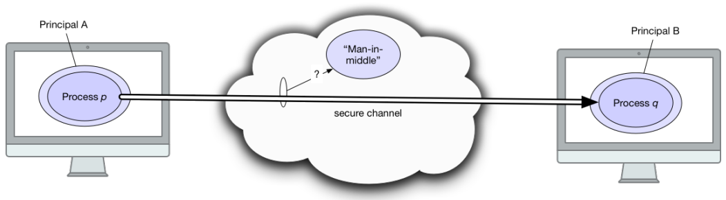
You also need to protect objects encapsulated by a distributed application.
This is called access control. Usually, access rights are associated with each principal (a user associated with an object, either the one requesting it or the one who owns it)

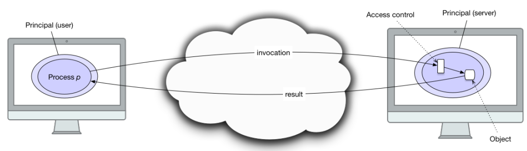
For example, XACML policies are enforced at the server based on the identity of the client.

Encryption and access control are great, but they don’t address DoS attacks.
Also, how do we deal with mobile code? How do we trust it?

Digitally signed code?
Run it in a sandbox?

I don’t know. I just write the notes.

Distributed Object Systems

Distributed OOP

There’s a thing called RMI (Remote Method Invocation).
Basically, you call methods on remote objects, as if they are local.
It’s crap and it’s not used anymore. But you still need to learn it to pass the exam see the advantages of other more modern approaches :)

The server sets up a bunch of remote objects and make their references accessible.
The client obtains remote references and invokes methods.
Java.rmi package gives programs API to perform these kinds of RMI operations.

Remote references are passed by parameters
Clients have proxies, or “stubs”, that allows clients to communicate with the server.
Java objects are instantiated from a compiled class, so RMI has to load classes from remote sites. It needs serialization and transmission of class specifications.

There are two fundamental concepts of RMI:

Remote object reference - so the client can talk to the server
Remote object interface - so the client knows what to do with the remote object

Remote Interfaces

There is an interface called Remote.
If an interface extends Remote, it can become a remote interface.
The methods in a remote interface can be accessed remotely.
Any object can be a remote object if it implements a remote interface.

A stub is a proxy for a remote object.
The stub implements the same methods as on the remote interface.

RMI middleware consists of:

Stub
Dispatcher (uses Java reflection, it invokes the remote method)

A remote implementation should:

Implement a remote interface
Require an appropriate constructor
Must provide behaviour on all methods on remote interface (obviously, you need to do that in Java anyway)

Server Deployment

To deploy an RMI server, you need to run the server itself, and you need a registry.
What’s a registry? It’s a separate instance of the JVM that maps URLs to remote references.
Yes, you need two Java instances to run an RMI server.
You can bind URLs using the bind method, as well as unbind and rebind.

Dynamic Code Loading

How do you trust the code that’s coming to your computer?
You need two things:

Security Manager - enforces rules, or policies
Security policy - the actual rules to abide by

A security manager, in Java, is stored via a singleton pattern (sort of).
You can set one up with System.setSecurityManager and access it with System.getSecurityManager.
So then how do you set up security policies?
You can use System.setProperty, or via the -D switch when initialising the JVM.

You also need a policy file, to store your policies.
The format looks a little like this:

grant {
permission java . net. SocketPermission
"*:1024 -65535",
"connect,accept,resolve";
permission java . net. SocketPermission
"*:80", "connect";
};

Many Clients!

How does RMI manage multiple clients running the same methods?
It opens up a new thread for each request!
But then we’ve got lots of threads acting on the same resources. If you’ve read the PLC notes, you know that this is a recipe for race conditions.
But in case you haven’t started PLC yet, a race condition is when two or more threads try to manipulate a shared resource at the same time.

So then, what do we do to stop race conditions from screwing things up?
We use a schedule! So that thread activities can be controlled.
Basically, we only want one thread trying to access a critical region (some mutable shared resource) at a time. This is called atomicity.
Also, when other threads try to access an occupied critical region, it’ll wait for the “lock”. This is called guaranteeing mutual exclusion.

In Java, there exists an implementation of the monitor concept.
A monitor is a barrier securing a shared resource with a lock.
When a thread accesses a shared resource, it gets the lock.
When more threads try to access the shared resource, it has to wait in queue until the lock is released.

The Monitor

Don’t worry! There’s not some weird class you have to use to use monitors.
You’ve actually been using monitors this whole time: it’s from the synchronized keyword.
It can declare critical regions of methods or objects.
When a thread tries to access code encapsulated with a synchronized block, it needs a lock of that object (or class, if it’s a static method).
For more information, read the PLC notes. PLC does a great job of covering concurrency!

The Observer Pattern

There’s also an observer pattern used for concurrent threads:

wait() - the thread stops and waits to be notified
notify() - wakes up a random thread
notifyAll() - wakes up all threads

This is more useful for scenarios such as the producer consumer problem.
Again, this is explained further in the PLC notes, so for more information, please check those.

RMI Limitations

Despite how amazing RMI is, it has disadvantages.
For example, it assumes both the client and server run in a JVM.
It doesn’t work if either server or client are not written in Java. For example, it can’t work with legacy code in COBOL, servers written in Python or C (good luck to you if you write servers in C) or a web application written in JavaScript.
You can use JNI (Java Native Interface) in some cases, but it’s a pain to work with (even more than RMI) and doesn’t always work.
It makes remote calls look like local calls, i.e. it assumes that the network is always reliable. Obviously, that’s not the case and it’s a pain to handle network problems with RMI.
All in all, RMI is a tightly coupled system. We don’t want tight coupling though, as we want to build servers and clients which are independent of each other, i.e. don’t restrict or affect each other.

So yeah, it’s clear: RMI sucks. Well, it’s not that it sucks; it’s outdated technology. Nowadays, we have things like REST APIs, which pretty much run the entire Internet.

Data Serialisation

Serialising Java Objects

In RMI, we send objects over networks, like parameters and stuff.
How do we do that?
The object needs to implement the Serializable interface!
If an object implements the Serializable interface, the compiler generates bytecode to handle serialization/deserialization.
The same version of the class must be known on both sides.
Objects are passed through networks using ObjectInputStreams and ObjectOutputStreams, with the methods readObject and writeObject.
You also need a version UID, because that’s important in sending objects over a network.

Mobile code 📱

We can use serialisation to create mobile code:

Client sends a message object to a server that contains behaviour
Server calls a method on the received object to execute the behaviour
The message object can then either be sent back to the client or visit the next server.

To do this, you can define an interface for tasks, called Task:

public interface Task extends Serializable {
public Object execute();
}

Then, you can create tasks that implement Task and send those to a server.
For example, you could make a LetterCount task, which has a string as a property, and the execute implementation could count the number of characters in the string and return the result.
If the client sent that to the server, the server could run execute and do something with the result (e.g. send it back to the client).
This is one way to send mobile code in Java, although it’s a bit hacky because the server must already be aware of the code in the first place; code isn’t actually being “transmitted”.
However, if you store a Task as a property in some ExecImpl class and send that, you could send code that isn’t preprogrammed into the server.

Pass by reference or value?

With serialisation, we’re passing a copy of the object.
However, with RMI, you can pass a reference of an object, using the Remote interface!

Let’s use an example with Banks and Accounts.
The Bank implementation passes references to remote account objects.
Both the client and the server have copies of the same Account object reference.

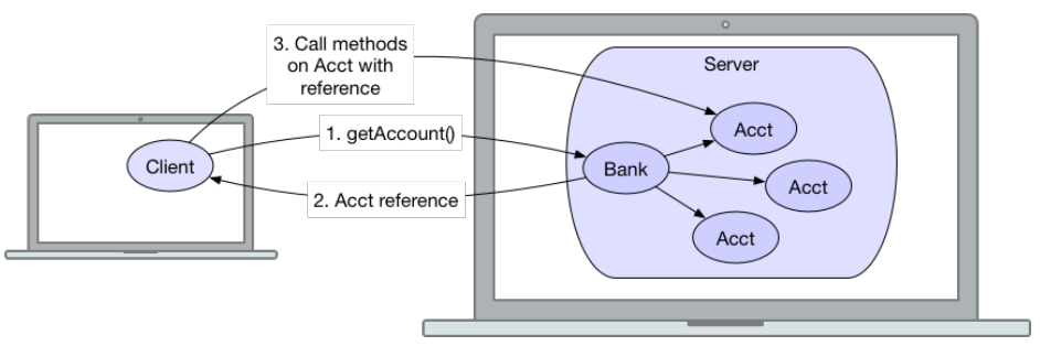
We can go further and use callbacks.
With callbacks, we pass a callback object reference (from client to server).
Basically, a client sends the server a request and some callback object.
Then, once the server has done performing the request, it uses the callback object, so the client can react to what the server has done.

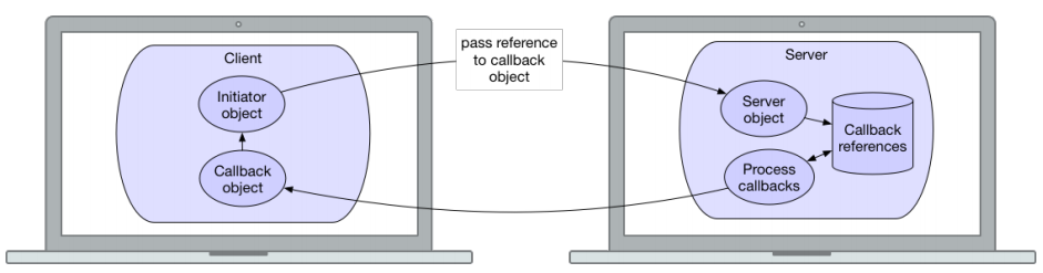
With RMI, the client’s calling thread waits until the remote method returns.
Callback allows decoupling between client and server.

Programming language independence

Don’t like the way Java is serialising your objects?
What was that? You wanted your Java programs and your C programs and your FORTRAN programs and your COBOL programs to talk to each other through a language-independent format?
No worries! Just override the writeObject and readObject methods and you can define your own language-independent format!

import java .io. Serializable ;
import java .io. ObjectOutputStream ;
import java .io. ObjectInputStream ;

public class MyClass implements Serializable
{
private static final long serialVersionUID = 2L;

private void writeObject ( ObjectOutputStream out )
throws IOException
{ // Custom solution
}

private void readObject ( ObjectInputStream in )
throws IOException , ClassNotFoundException
{ // Custom solution
}
}

But that’s effort! You want to use a standard because you’re lazy and don’t want to define your own format yourself you’d also like to support other programs, and using a well-defined standard makes everything easier.

So what should the standard have?

Syntax: What is the structure of the byte stream?
Semantics: What do the symbols mean?

JSON

JSON (JavaScript Object Notation): a language-independent syntax for exchanging structured data
There are three main components:

Value: a number, a string, a boolean, an array, an object or null
Array: a list of values [ ]
Object: a mapping from keys (written as strings) to values { }

For example, here is a JSON document expressing an auction structure, containing items with IDs, names and stock:

{

“auction”: “Notes Network Auction”

“items”: [

{

“ID”: “023469234”,

“name”: “Red Stone of Aja”,

“stock”: 1

{

“ID”: “FE40536”

“name”: “String”

“stock”: 58

{

“ID”: “296360”

“name”: “Time Stop Hat”

“stock”: 3

]

}

JSON documents should be underpinned by schema (semantics, or set rules) which can be defined by a “$schema” or/and “$id” property.

GSON

GSON is a JSON helper API made by Google.
Basically, it lets you use JSON in Java.
It has reflection-based functionality, which allows it to convert Serializable objects into JSON and back again.
If you wanna check out more, look at the repo: https://github.com/google/gson

Linked Data & Semantics

There’s a method of encoding linked data to JSON called JSON-LD.
It’s a W3C recommendation (standard) to use this.
It uses a common schema with defined relations, most of which can be found here: https://schema.org/ (such as sameAs, is-a, requires, attachedTo etc.)

We can also use this to describe policies for distributed systems, not just with access control, but for behaviour control, too.
The International Labour Organisation reported fatalities in low/middle income countries due to workplace accidents and illnesses. This was because equipment didn’t comply with OHS policies.
So they used W3C SSN Ontology for sensor descriptions and a framework called OWL-POLAR for semantical policy representation, and now it’s being used in coal mining.

Also, if we can describe things, rules, policies, we can describe networks, too. That’s called software-defined networking, and we’ve already seen a bit of that already (with virtual LAN).

Loose Coupling

Space & Time Uncoupling

If senders and recipients don’t have to be directly connected to each other, we are decoupling with space.
If sending and receiving messages can happen at any time anyone is available, we are decoupling with time.
This can make one-to-many communication easier.

Here are the effects of coupling:

Time coupled

Time uncoupled

Space coupled

Message is directed specifically towards receiver.

Receiver must be present when the message is sent.

Example: sockets, remote invocation

Message is directed specifically towards receiver.

Receiver doesn’t have to be present when the message is sent.

Example: snail mail (normal mail), email

Space uncoupled

Sender doesn’t know exactly who they’re sending to.

Receiver must be present when the message is sent.

Example: IP multicast

Sender doesn’t know exactly who they’re sending to.

Receiver doesn’t have to be present when the message is sent.

Example: publish & subscribe with message queues

Group Communication

A sender sends a message to a group
All the recipients of that group receive the message
Participants may leave / join the group
A single multicast operation is used for sending the message
Usually implemented with IP multicast

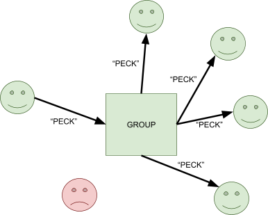
The frowning person won’t receive the message as they aren’t available, hence why this is space-uncoupled-time-coupled.

You can think of this as a space uncoupled time coupled network (assuming there aren’t any message queues).
You can use this to send information to a large number of clients, or in a collaborative application.
It’s also handy for different kinds of groups, such as closed groups (where only members can send messages) or open groups (where any process can send messages).

There are two kinds of group communication:

Synchronous group communication: the messages are sent out in real-time, and bounds must be set on communication delays, process scheduling delays and faulty components.
Asynchronous group communication: messages are sent via datagram (UDP), so they may get lost, so systems are characterised by communication uncertainty. We should set bounds of timeout delays and assume timely communication most of the time.

When implementing, we need to ensure:

Reliability: message received is identical to the one sent (integrity), every message is eventually delivered (validity) and if a message is delivered to one member, it’s delivered to all (agreement).
Ordering: sender order is preserved (FIFO), and can either have:

Causal ordering: just make sure if message m2 is sent in response to m1, m2 is received by all members after m1.
Total ordering: all messages are sent in the same order, regardless of causality.

Remember that we also need some kind of management, so we can create/delete groups, add/remove participants, detect failures and notify members of membership changes.

Publish & Subscribe

Publish and subscribe is the most widely used form of indirect communication.
Also known as distributed event-based systems
Basically, publishers publish events to an event service, and subscribers express interest (or subscribe) in particular events.
It’s like a special kind of group communication, also making this space-uncoupled-time-coupled (assuming that the system doesn’t store any events).
These kinds of systems deliver event notifications.
Publishers can also publish messages by topic, and subscribers may want to subscribe to a set of topics.
If a subscriber is not running, events may be stored and queued until it rejoins.
When events are queued, the system becomes time-uncoupled since it will store them until a subscriber comes back online
You’ve seen lots of these before, like:

Subscribing to a channel on YouTube (except you actually get told when they upload)
Financial information systems (like the stock market)
Cloud-based workflows
Cooperative working systems

An example of an infrastructure that uses pub & sub is Google Cloud Pub / Sub (creative name).
It supports many-to-many communication, and it has heterogeneity, which means it supports different components written by different developers.

The types of subscription models are:

Channel-based: subscribers subscribe to a channel, so they receive all events
Topic-based: subscribers subscribe to a set of topics, so they only receive messages sent to those topics
Content-based: subscribers filter messages based on queries, and only receive those.

The types of implementation models are:

Centralised: A single publisher sends messages to multiple subscribers via point-to-point messages (it lacks resilience and scalability)
Distributed: A network of publishers work together (also called federated)
Peer-to-peer: Some fully peer-to-peer implementations are possible

Message Queues & IoT

That’s great, but we still don’t have full decoupling (unless we store events); how do we decouple time, too? Do we need a time-based stand, like Killer Queen or King Crimson?
No, using message queues are enough.

Traditionally, message queues are point-to-point services.
Senders (or producers) place messages into queues, and receivers (or consumers) take messages from the queues.
This way, producers and consumers can have different lifetimes, decoupling time. It’s also suitable for enterprise applications.

What protocol uses message queues like this?
There’s one called MQTT (Message Queue Telemetry Transport), and it’s very light-weight! Perfect for embedded systems, edge computing and Internet of Things.

Why not just use HTTP? Well, HTTP is better for requesting information. Plus, it’s not event-oriented and it can be more bulky than MQTT.
However, the way MQTT defines its namespaces is similar to HTTP, as it uses a hierarchical system.
The sub-topics are separated with “/”, and it gets more specific as you specify more topics.
For example, some device could publish to:

<town>/<postcode>/<house>/alarm
<town>/<postcode>/<house>/temperature
<town>/<postcode>/<house>/energyUse

... and subscribe to:

<town>/<postcode>/<house>/thermostat/setTemp

Subscribers can also use wildcards:

Single-level wildcards “+” selects every topic at that hierarchy
Multi-level wildcards “#” selects every topic path
For example:

Southampton/+/+/energyUse - subscribe to energy use for all homes in Southampton
Southampton/SO171BJ/# - subscribe to all queues for all homes in SO17 1BJ

It’s also cheaper to maintain a MQTT connection than a HTTPS connection, as it requires less power:

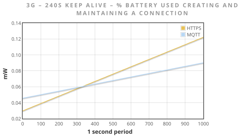
A subscription can either be:

Durable: messages are stored until next time subscriber connects
Non-durable: messages remain as long as subscriber is connected

Publishers can also make publications “retained”.
This means that “last known good” messages are sent to new subscribers.

MQTT is really small; the smallest packet size is 2 bytes! It’s compressed into bit-wise headers and variable length fields.
It has asynchronous bidirectional pushing, so no polling.
It supports always-connected and sometimes-connected models
It’s aware of sessions, and usually operates over TCP.
Plus, the sender and receiver can agree on a quality of service (QoS) based on a 2-bit integer:

0 - messages are delivered at most once
1 - messages are delivered but may be duplicated
2 - messages are delivered once and only once

Because MQTT is so minimalistic, it’s perfect for devices with limited resources, like game controllers or small battery powered devices.
Implementations of MQTT are available for C and Java, but one of the most popular is one called RabbitMQ.

RabbitMQ

RabbitMQ is a multi-protocol implementation that is polyglot (supports multiple languages).
It supports:

AMQP (Advanced Message Queuing Protocol) - message-oriented pub/sub queueing protocol with reliability and security
MQTT (Message Queue Telemetry Transport) - pub/sub based protocol designed to be minimalistic for small code footprints
STOMP (Simple Text-Oriented Messaging Protocol) - similar to HTTP and has commands such as CONNECT, SEND, SUBSCRIBE, UNSUBSCRIBE

Since it is polyglot, it supports many languages, for example, you could write the producer in Java and the consumer in Python.

It also supports different communication patterns, such as pub/sub, topic-based routing and RPC (Remote procedure call).

Distributed Transactions

Distributed Data

When you distribute data, it needs to follow the ACID rules:

Atomicity: either a transaction happens or not at all
Consistency: a transaction takes the system from one consistent state to another
Isolation: effects of a transaction are not visible until it’s fully complete
Durability: effects of a transaction are persistent (resistance to failures)

To put this into context, we need:

objects to be recoverable
clients to signal the start/end of a transaction
commitment processes to guarantee all operations are permanently recorded
the protocol to ensure aborted transactions leave no visible effects

We need some kind of Coordinator to uphold these rules...

Lost Updates & Inconsistent Retrievals

Here are two kinds of problems we could face:

Lost updates

This is where an update is lost by transaction U because transaction T overrides it:

Transaction T	Transaction U
bal = a.getBalance(); $200
	bal = a.getBalance(); $200
	a.setBalance(bal * 1.1); $220
	commit
a.setBalance(bal - $100); $100
commit

As you can see, the final value is supposed to be $120, but because T accessed the value before U changed it, it sets the balance to $100 instead. The update of U was lost!

Inconsistent retrievals

This is where a transaction U doesn’t get the right value from a retrieval because they’re trying to access before transaction T is finished:

Transaction T	Transaction U
a.withdraw($100); $100
	total = a.getBalance(); $100
	total += b.getBalance(); $400
b.deposit($100); $400
commit	commit

The problem here is that when U gets the balance of account B, it shouldn’t be $400, it should be $500, because T wanted to deposit $100 into B.

So how do we fix this?
Serial equivalence!
What is that? That means to ensure serially-equivalent interleaving, as if the transactions happen one after the other.
This prevents lost updates and inconsistent retrievals.
So how can we serialise them?
Two ways:

Locking: transaction must acquire a lock on an object before they act on it. Other transactions must wait for the lock, but can share a read lock. This could lead to deadlock.
Optimistic concurrency control: perform the transaction anyway, and if we have a conflict at the commit stage, then abort. It’s similar to CAS (compare-and-set) in PLC.

But what if we want to abort transactions? Then we’ll have new problems!

Dirty Reads & Premature Writes

Here are two problems we could face with aborting:

Dirty reads

This happens when transaction U happens after transaction T, but then transaction T wants to abort after U has already committed, which makes U’s read “dirty” (because it’s not accurate anymore):

Transaction T	Transaction U
bal = a.getBalance(); $200
a.setBalance(bal * 1.1); $220
	bal = a.getBalance(); $220
	a.setBalance(bal + 20); $240
	commit
abort

As you can see, T aborts after U is finished. That means U’s read of account A’s balance is now dirty.
We need recoverability, and to avoid cascading aborts by delaying reads until other transactions commit or abort.

Premature writes

This happens when a write happens just before a transaction aborts and rolls back a data value:

Transaction T	Transaction U
$200
a.setBalance($250); $250
	a.setBalance($220); $220
	commit
abort

If T is aborting, A’s balance should be $220, right?
What if the implementation of an abort is to roll back the previous balance?
Then the result would be $200! Not good!
To fix this, we can delay writes until earlier transactions that update the same objects have committed / aborted.

Remember that communication is not fully reliable; it can crash, or links may temporarily fail.
Some transactions may be affected by this. What will we do? How will we recover?

You think Bart Simpson from the slides will care if your transactions are fully committed? Probably not.

Distributed Commit Protocols

So we need atomicity - all or nothing
We need durability - account for failures
We need locks on all data objects involved
Hmmm... how about a distributed commit approach?

Who’s going to coordinate? Use a leader election protocol!
Shall we commit or abort? Use a consensus protocol! (more info in Corina’s bit)

Basically, a coordinator asks a bunch of participants if they want to commit.
They all commit if everyone else says they’re ready to commit. This is called Single Phase Commit.
The coordinator keeps asking until everyone acknowledges.
But how long do we wait, and what happens if some participants fail?

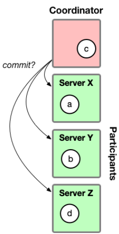
Two-Phase Commit

Two-phase commit is a voting scheme to reach a consensus on whether to commit or abort.
It preserves atomicity, because if one operation is aborted the entire transaction is aborted.
This scheme requires a reliable message delivery.
The servers can all abort their own operations if the coordinator can detect it.

It’s split into two phases:

Voting

The coordinator sends instructions to all participants and asks them if they can commit.
For all participants, they execute the instructions and if they can commit, they respond with YES and save state to local storage. If they can’t commit, they respond with NO and abort local operations and release locks.

Completion

The coordinator collects all the votes (including its own).
If all the votes are yes, the coordinator sends a doCommit message to all participants, and all participants send back a haveCommitted message.
If even a single vote is no, the coordinator sends a doAbort message to all participants, and everyone aborts.

2PC Failure Handling

That’s great, but how does it handle failure?

If a participant crashes after voting yes, the participant saves its state to local storage and uses that to reinstate an equivalent participant. Then, it will call getDecision on the coordinator and will use that decision to either commit or abort.

If a coordinator crashes in phase 2 (completion), 2PC can become a blocking protocol.
Participants can’t use getDecision, because the coordinator is gone. What are they going to do?
They need to elect a new coordinator using a leader election protocol! The new coordinator issues an abort message.
Recovery can take time (obviously).

Increasing Concurrency & Deadlocks

How do we increase concurrency in our system?
Objects can have multiple locks!
This is called Two Version Locking.
Here’s the basic principles: every object has three locks: read, write and commit. If you have a respective lock on that object, you can perform that action.
Threads can share locks too, for example multiple threads can share the read lock on an object.
However, some locks are unobtainable while other locks are already set.
For example, if the write lock has already been set, another thread needs to wait to also obtain the write lock.
The full table is here:

	Lock requested
Lock already set	Read	Write	Commit
None	OK	OK	OK
Read	OK	OK	WAIT
Write	OK	WAIT
Commit	WAIT	WAIT

Following the table, if the “read” lock is already set, it’s alright to share the read lock or take the write lock (if the write lock isn’t already taken).
If multiple locks are taken, the strongest (bottom-most) lock takes precedence on the table.
As you can see, while an object is being committed to, no-one can do anything with it until after it is finished.
However, it is possible to have many readers and a single writer, since setting the write lock doesn’t stop threads from reading the object.

The advantage of this is that read operations are only delayed during commits.
However, read operations on one transaction can delay commitment on others (since all reading and writing needs to stop during commitment).

There’s still one problem though: deadlocks!
We still have the overhead of checking and maintaining deadlocks.
We can break them using timeouts or probes.

Distributed Systems Theory (Corina)

Time in Distributed Systems

Clock synchronisation

Distributed systems need to sync up!
If they don’t, messages could arrive out of order. Sometimes that can be disastrous!
In practice, this is mostly used in things like banking or e-commerce.
There’s no way to be fully synchronised, but there are two methods of synchronisation:

External synchronisation: all processes are synced up to some external clock, like UTC
Internal synchronisation: processes use some kind of sync protocol to sync up their local clocks with each other. They agree on a common time, but not necessarily a standard (like UTC)

To achieve internal synchronisation between two processes, process A sends its time to process B in a message. Then, B sets its own time to , where max is the maximum time needed to transmit a message, and min is the minimum time needed to transmit a message.
Basically, your time is the other process’ time plus the average time to transmit a message.
In asynchronous systems, max isn’t known!

But what if you wanted to have internal synchronisation with multiple processes?
You can use the Berkeley algorithm!
It works like this:

One machine is chosen as the master.
The master then periodically polls everyone’s clock values.
The master then estimates local times based on round trip times, and then averages (fault-tolerant average that disregards faulty clocks) out the values (including the master’s own time)
The master then sends the amount by which processes need to adjust their individual times (not the new clock value!)

For external synchronisation, you can use Cristian’s algorithm.
The way that works is as follows:

There is a process and a time server.
The process requests for the time, , from the time server.
The time server responds to the process with the time, .
The process then sets its own time to , where is the time taken by the request and reply.

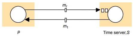
Why add that bit at the end? Well, by the time the time server responds with T, T is no longer the time anymore, because of the time spent waiting for the message to get to us. That’s why we estimate how long that message took, and we add it to the time we receive.
Admittedly, this assumes the time to request and receive are distributed evenly.

There’s another synchronisation method called Network Time Protocol (NTP).
NTP allows clients to be accurately synchronised to UTC.
It works in a hierarchy system, with:

primary servers (at the top) directly connected to time source (e.g. radio clocks)
secondary servers which synchronise with primary ones
tertiary servers which synchronise with secondary ones
etc.

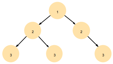
The time is synchronised down the hierarchy using multicast, or Cristian’s algorithm.
A client is somewhere in this hierarchy, and the lower they are in the hierarchy, the less accurate the time they’re synced with is.

Logical clocks

Some distributed algorithms only care about the ordering of events. That’s where we use logical clocks.
Logical clocks use event causality to obtain partial ordering of events.

Alright, so how do we get causal ordering with logical clocks?
First, we define a relation , where and are events:

If and are events in the same process and a occurs before b, then
If is the event of sending a message and is the event of receiving the message, then
Transitivity rule: if and then
This relation is called the “happened-before” relation (a happened before b)

We assume that holds, even if it doesn’t make much sense
Messages and are concurrent if neither nor . That’s written as .
Here’s an example:

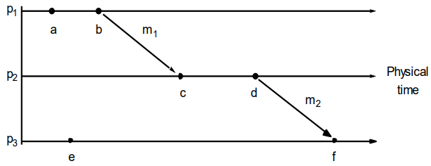
is true because and happen in the same process, and happens before .
is true because is a send event and is that respective receive event.
is true because of the transitivity laws.
is also true because and are both false (you can’t derive them).
There are other causalities too, like , , and .

We can capture this concept numerically, with Lamport’s Logical Clocks.
Basically, each process keeps their own logical clock, starting at 0.
When a process sends or executes an event, it increments its logical clock and timestamps it, so the recipient can see the timestamp.
When a process receives an event, it checks if the timestamp received is bigger than its own clock. If it is it first sets its own clock to the timestamp and then carries on with the same procedure described above.
This may be a little hard to visualise at first, so let’s use an example:

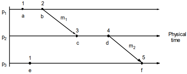
Below, I give an explanation to all the timestamps of the events:

a - process 1’s first message, so it has a timestamp of 1
b - process 1 has already executed event a, so the clock of process 1 was incremented by 1, to make it 2. When process 1 executes b, it’ll be timestamped with 2, because that’s process 1’s clock value at that moment.
c - process 2’s clock is 1, but the timestamp of the message is 2. The message’s timestamp is bigger, so process 2 will increment and use that one for c. Incrementing 2 gives 3, so the timestamp of c is 3.
d - process 2’s new clock is now 3, because of event c. The clock will be incremented and used to timestamp d, so d’s timestamp will be 4.
e - process 3’s clock is still 1, and has no events yet. So process 3’s first event, e, will have a timestamp of 1.
f - process 3’s clock is 2 after event e, and the timestamp of the message from d is 4. The message’s timestamp is clearly bigger, so that will be incremented to 5 and used for the timestamp of f.

To refer to the timestamp of an event, use .
implies
... but does not imply , because could be concurrent to ()

In the example, a and e have identical timestamps. How do we differentiate them?
We use Totally Spies Ordered Logical Clocks!
All we have to do is add the process ID to the event timestamp.
So instead of something like 1 for event a (in the example above), it would instead be (1, 1), or (3, 2) for c, or (5, 3) for f.
is true if:

or and

For example, under total order in the above example, a < e because (1, 1) < (1, 3).

What if we wanted that implies rule to be true?
With vector clocks, that can be arranged!
Instead of an integer being stored as a clock, a vector is stored instead.
Instead of incrementing an integer value, the process increments its own field in the vector.
It works almost the same as normal logical clocks, except we’re using vectors instead, and each process has their own field in the vectors.
Upon receiving a message, it updates all the fields of it’s own clock with the newly received clock if it’s bigger than the one we already have (more formally, for all j)
When we compare vectors:

iff for all
iff for all
iff and

It’ll be easier to show an example again:

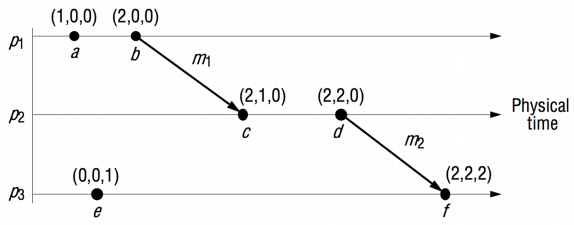
Below, I give an explanation to all the timestamps of the events:

a - process 1’s vector clock is empty, (0, 0, 0), so process 1’s slot (the first slot) is incremented to (1, 0, 0) and is used to timestamp a.
b - process 1 increments their first slot again to get (2, 0, 0) and uses that to timestamp b.
c - upon receiving the message from b, it updates all the slots in its own local clock with the slots in event b’s clock (only if it’s bigger than what we already have). Process 2’s clock is currently (0, 0, 0) and event b’s clock is (2, 0, 0), so the first slot will be updated with ‘2’ in process 2’s local clock. Now, process 2 increments its own slot (the second slot) to (2, 1, 0) to use for event c.
d - process 2 increments their own slot again to get (2, 2, 0) and uses it for event d
e - process 3’s vector clock is still empty, at (0, 0, 0). It increments its own slot (the third slot) to (0, 0, 1) and uses that for event e.
f - process 3 updates its own clock, (0, 0, 1), with the new clock from event d, (2, 2, 0). The first two slots are clearly bigger, so process 3’s clock is updated to (2, 2, 1). Process 3 then increments its slot to (2, 2, 2) to use for event f.

With vector clocks, we can not only see the number of events a process has timestamped, but we can see how many events another process has executed that affected some other process.
What’s also good about vector clocks is that implies .
Why? If , that means all the slots in event a’s clock is smaller than or equal to every slot in event b’s clock, and slots can only go up (they can’t be decremented), so a has to have gone before b.
If , then events a and b are the same events, just different names. We’ve already established that , so this is trivial.

The disadvantage to using this over Lamport timestamps is that storage and message payload is proportional to N (the number of processes), so it’d be inefficient to use this unless we have to.

Distributed Mutual Exclusion

Failure detectors

Failure detectors detect failure (wowee, now that’s what I call info)
There are two kinds of failure detectors:

Unreliable: returns either unsuspected or suspected hints (can only suspect if a process is no longer alive via an “alive” message not being received back)
Reliable: returns either unsuspected or failure (if it sends ‘failure’, it knows for sure a process is down)

Distributed Mutual Exclusion

You have some distributed critical region, and all the online processes wanna grab it and mess with it at the same time. Big no-no. You want them to take it in turns.
You want to do it with message passing.
We need to make some assumptions:

There are N processes
Network is reliable but asynchronous
Processes don’t fail
Processes spend finite time in critical section (they don’t hang while in critical section)

There are also some properties of mutual exclusion algorithms/protocols:

Correctness:

Safety: at most one process is in critical section
Liveness: requests to enter / exit eventually succeed
Fairness: access to critical section happens in happened-before order, so if action 1 is requested before action 2, then action 1 should go first and then action 2.

Performance:

Minimise number of messages sent in entry / exit operations
Minimise client delay (entering / exiting critical section)
Minimise synchronisation delay (time between one process exiting and another entering critical section)

So what kinds of algorithms are there?
Firstly, there’s the Central Server Algorithm.
It’s based on one server and many clients. Simple enough.
The server has a token, and clients can REQUEST for the token or RELEASE the token.
If a client requests for a token and it’s taken, they’re added to a queue to wait for the token.
It’s basically the whole lock concurrency ordeal, but in a distributed setting.

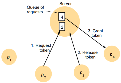
It has safety, because if the token belongs to a process, other processes can’t have it
It has liveness, because all requests are handled by a server, and all request messages are eventually answered once they’re at the front of the queue
It does not have fairness because there are no timestamps -- it’s an asynchronous system. For example, say that request #1 request #2. Request #2 could come earlier than request #1 and process #2 could get the token, when in reality it should’ve been process #1. See this slide for more detail.
This has good performance, but there is a single point of failure and the server acts as a bottleneck. That’s bad! But we can find a way around this...

Next we have the Ring-based Algorithm!
It’s essentially the same as the server based one, except without a server and it’s a ring.
Tokens aren’t explicitly sent to one process; it’s passed around a ring.
For example, when process 2 is finished with the token, it’ll pass it to process 3, who will pass it to process 4 and so on.

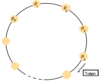
It has safety, because again, only the process with a token has access to the critical region.
It has liveness, because eventually everyone will get the token.
It does not have fairness, because the order of processes in the ring topology might not be the order in which we want the processes to act on the shared data.
We no longer have the bottleneck, but this’ll really weigh us down on bandwidth, as the token might have to travel quite far just to get to a process that needs it.

Why not use an algorithm using multicast and logical clocks?
There’s one called Ricart and Agrawala’s Algorithm which uses these in a very interesting way.
In this algorithm, messages have totally-ordered timestamps. Don’t think too hard about it; it just means that processes can tell when messages were sent.
When a process wants to access a critical region, it sends a REQUEST multicast message to all the participants.
When a process receives a REQUEST message, it can do one of two things:

If this process is already in the critical region, or if this process also wants to access the critical region but this process wanted to access it before the sender, then the sender of the request message is put in a queue
If the sender wanted to access the critical region before this process, then it will send a simple REPLY message to the sender. That’s all; no extra info in the message or anything. It’s sort of like a “sure, you can use the critical region as far as I care”

When a process gets REPLY messages from all other participants, it gets access to the critical region.
Confusing? Let me show you an example:

Image	Explanation
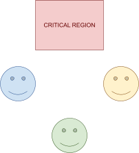
	We have three processes and the critical region.
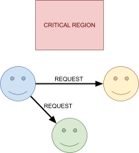
	The blue process requests access to the critical region from all other processes.
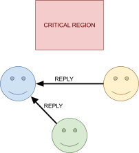
	Both the green and yellow processes don’t care about the critical region, so they both immediately reply to the blue process.
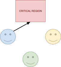
	The blue process, having received replies from all other participants, can now use the critical region.
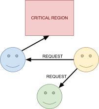
	Yellow wants to use the critical region now, so they send out requests to everyone.
	Blue adds yellow to their queue, because blue is currently using the critical region. Green doesn’t care about the critical region, so green replies to yellow.
	Now green also wants to use the critical region. They send out requests to everyone.
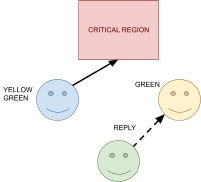
	Blue is using the critical region, so green is added to the queue. Yellow came first (it knows because of the totally-ordered timestamps), so yellow adds green to its queue.
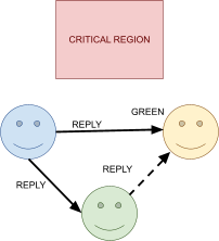
	Blue is now done with the critical region and sends a reply to yellow, because yellow was at the head of the queue. It will also send a response to green, because they’re next on the queue.
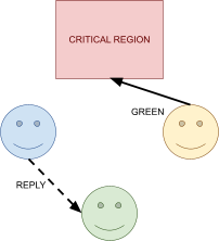
	Yellow just got responses from everyone! That means yellow can now use the critical region.
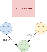
	Yellow is now done with the critical region, and sends a response to green. Green now has all the responses, and can now use the critical region.

This has safety because a process doesn’t reply if they are in the critical region.
This has liveness because the total ordering of the timestamps ensures each request will eventually get all replies, and because each participant spends finite time in critical section.
This has fairness because with the timestamps, whoever requests first will go first, and whoever requests after will go second and so on.
The performance is good because the token isn’t circulating.

Wow, this is, like, the perfect algorithm!
But what if I told you that we don’t even need all those replies from all those participants?
We can also use Maekawa’s Voting algorithm! (No, I don’t mean Maekawa from iDOLM@STER)
The whole gimmick of Maekawa is that we use groups instead of individual processes.
There’s one group for each process, and all the groups overlap each other, and each process needs to be in either 2 groups or more (if there are any less, then there’s no overlapping)
As for the size of these groups, an optimal amount would be (where N is the number of processes). In practice, this makes the groups non-trivial to construct, so we use a simpler method which has group sizes of :
Construct groups by first arranging the processes in a matrix, then work out the group for each process by taking the union of the row and column that it’s in. For example, these are the groups for A and B respectively in a situation with 9 processes.
This ensures that every pair of groups overlap.
The algorithm works like this:

For each process there is a group
For to access the critical region:

It must not already be voting for someone else
It sends REQUEST messages to all processes in its group,
It waits for VOTE responses from all processes in its group

For receiving a REQUEST from :

If is already in the critical region, or if they’ve already voted for someone else, then put in the queue.
Otherwise, send a VOTE message to .

For to exit the critical region:

It sends RELEASE messages to all processes in its group,

For receiving a RELEASE from :

If there is a request in the queue, take the first process out of that queue and send them a VOTE.
Otherwise, simply remember that we have no votes for anyone.

What? Still confusing? Let me illustrate it for you:

Image	Explanation
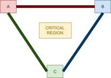
	We have participants A, B and C. The groups are: A’s group: A, B B’s group: B, C C’s group: C, A
	A wants the critical region, so it multicasts a REQUEST message to it’s group (B).
	B isn’t in the region, and it hasn’t voted for anyone else, so it’ll vote for A.
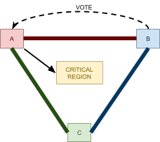
	Because A has received all votes from its group, it gets access to the critical region.
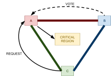
	Now C wants to access the critical region! It sends a REQUEST to its group (A).
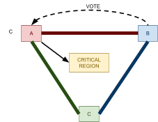
	However, A is already using the critical region, so it puts C in the queue.
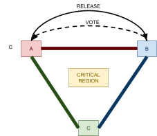
	A has now finished, and will send a RELEASE message to its group (B).
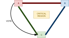
	B will now cancel the vote with A. A looks at the queue and sees that C tried to access the critical region. A will now vote for C.
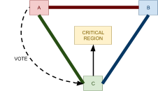
	C, now having all the votes in its group, now has access to the critical region.

So, how good is this one?
This has safety because a process needs all votes to enter the critical region, and other processes can’t vote for someone else if they’ve already voted for someone in a critical region.
This does not have liveness because deadlocks can occur.
This does not have fairness because there are no timestamps; processes can’t tell which requests should be served first (only via queue).
The performance isn’t even that much better than Ricart and Agrawala.

So why does this have deadlock?
Because we can create a chain of reply waiting!
In the example above, if everyone wanted to use the critical region, we could have this as a deadlock:

A is waiting for B’s reply
B is waiting for C’s reply
C is waiting for A’s reply

To solve this, we could incorporate timestamps into the requests to give order to the requests.

All of these algorithms are great, but they don’t tolerate message loss.
When processes crash, what happens?

The ring-based algorithm just stops working altogether
Some crashes are tolerated by central server and Maekawa
Ricart and Agrawala can be adapted to tolerate process crashes, assuming a reliable failure detector is available

Leader Election

Why use election algorithms?
Sometimes we want to elect a coordinator amongst a bunch of participants.
Everyone has to agree on one, so how do we do it? Election algorithms!

We need some assumptions first though:

There are N processes with unique, totally ordered identifiers
Process with the largest ID must win election (for these examples, this condition will be different in practice)
Messages are eventually delivered (no failed packets)
Each process can call only one election (unless coordinator fails)
Multiple concurrent elections can be called by different processes
Participant: process engaged in an election
Each participant has a variable initially

Wait! One more thing! How do we determine correctness and performance, like in the distributed mutual exclusion algorithms?
Correctness:

Safety: a participant’s elected vote is either nothing or P where P is the non-crashed process with the largest identifier
Liveness: all processes participate and eventually set their elected vote to something other than nothing or they crash

Performance:

Minimise total number of messages sent
Minimise turnaround time (number of serialised message transmissions in a single run)

Asynchronous systems

With asynchronous systems, we use a ring-based algorithm.
In this, all processes are gathered around in a ring.
A process sends messages to the process next to it in the ring.
This can only work with no process failures!

This one’s actually quite simple. Here’s how it goes:

Initially, every process marks itself as a non-participant.
Any process can call an election by:

Marking itself as a participant
Places its ID in an ELECTION message
Sends that message to its neighbour

For receiving an ELECTION message:

If message ID > our ID, forward the message and mark ourselves as a participant, if we’re a non-participant.
If message ID < our ID:

If non participant, replace ID with our ID, forward message, mark ourselves as participant
If participant, stop forwarding (should only happen when doing multiple elections)

If message ID = our ID, then we’ve found our coordinator. Set our elected variable to our ID, and send an ELECTED message with our ID to our neighbour. Set ourselves as a non-participant.

For receiving an ELECTED message:

If message ID != our ID, set our elected variable to the message ID and pass it along. Set ourselves as a non-participant.
If message ID = our ID, stop forwarding (because we know we’ve hit full circle).

To make this work, lots of processes should instigate elections, but this example will show you just one so you understand the algorithm (it is worst-case):

Image	Description
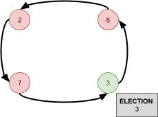
	We have processes 2, 6, 7 and 3 in a ring. 3 decides to start an election and creates an ELECTION message with 3 in it. It passes it to its neighbour. Red = non-participating Green = participating
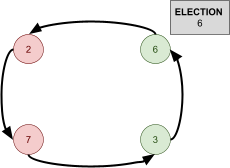
	6 receives the message and sees that it’s ID is bigger than the one in the message. It puts its ID in there, sets itself as participating, and sends the message to its neighbour.
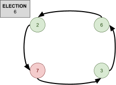
	2 receives the message. 2 is smaller than 6, so it just forwards the message and marks itself as a participant.
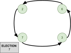
	7 receives the message. 7 is bigger than 6, so it replaces the ID, forwards it and marks itself as a participant.
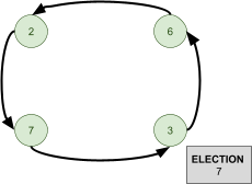
	3 receives the message. Since 3 is already a participant, and 3 is smaller than 7, it’ll just forward on the message. In fact, 6 and 2 will just forward on the message too. It’ll only differ when 7 receives the message, so we’ll skip 2 and 6 for now.
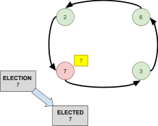
	7 receives the message. Since it’s already participating, and the message ID is equal to 7’s ID, it realises that they are the new coordinator. It creates an ELECTED message with it’s ID in it, sets itself as 7’s elected process, and sends the ELECTED message to its neighbour. 7 will also mark itself as a non-participant.
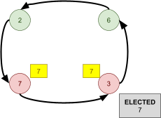
	3 receives the ELECTED message. 3 is not 7, so it sets 3’s elected process as 7 and forwards the message. 3 will also mark itself as a non-participant. 6 and 2 will do the same thing, so again, the algorithm only differs when the message goes to 7.
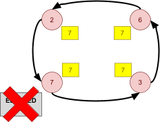
	7 receives the message. The ELECTED message ID is equal to 7’s ID, so 7 stops forwarding the message and the message is “deleted”. A new coordinator has been elected with all participants!

So how good is the ring-based algorithm?
It has safety, because only the process with the largest ID can start an ELECTED message
It has liveness, because eventually every process becomes a participant and receives ELECTED messages

Best case

Worst case

The initiating process has the highest identifier.

There are N ELECTION messages...

... and N ELECTED messages...

...resulting in 2N turnaround messages (messages sent in total)

The anti-clockwise (last) neighbour has highest identifier.

There are 2N - 1 ELECTION messages...

...and N ELECTED messages...

...resulting in 3N - 1 turnaround messages (messages sent in total).

This works best if more than one process starts an election, because you’re more likely to get that best case!

However, this algorithm does not tolerate failures.
Can we modify the ring-based algorithm to support failures?

Introducing the modified ring-based election algorithm!
Broken links are detected by the message sender and the ring is repaired (by making the next node your neighbour or something)
Basically, the messages now carries a list of processes that have forwarded this message.
An ELECTION message is started by the initiator and goes full circle once, tracking IDs. After it goes full circle, a new coordinator is selected from the list of processes and an ELECTED message is pushed around, just like the normal ring-based algorithm (except we’re still tracking IDs).
When the ELECTED message reaches the initiator of the election, it checks if the coordinator appears in the ID list.
If it does, then the election was successful.
If not, then another election is started.

Ring-based algorithm message	Modified ring-based algorithm message

Well? What’s good about this one?
For starters, it requires fewer messages (2N at most) and it tolerates failures.
However, the messages are larger.
If two processes initiate concurrently, then we can discard the message sent by the lower ID initiator (we could change it so that the message could remember who initiated the election).
If an initiator fails, the successor to the initiator can notice when the message went all the way around by spotting its own ID in the list of IDs in the message. Then it can act as the new initiator.

Can we have a totally correct election algorithm for fully asynchronous systems?
We actually can’t, because election algorithms can solve consensus, and as you’ll see later, there exists no consensus algorithm for any asynchronous system.
If that’s so, then the modified ring algorithm shouldn’t work. What’s wrong with it?
It’s good in theory, but in a real asynchronous system, you can’t truly detect leader failures or repair the ring (how do you know who will replace your neighbour?).

Synchronous systems

With synchronous systems, we use a bully election algorithm.
The bully algorithm has a few assumptions:

Processes can crash and restart
Message delivery is reliable
It’s a synchronous system, so we can use timeouts
Each process knows all other processes and can communicate with all
Each process knows which processes have higher IDs

The whole point of the bully algorithm is to select a new non-failing coordinator.

The algorithm goes like this:

If process P recovers from failure, or detects that the current coordinator has failed:

If P has the highest ID, it sends a COORDINATOR message to all other processes
Otherwise, P sends an ELECTION message to all processes with a higher ID than itself

If P receives no ANSWER message after sending an ELECTION message, it declares itself the new coordinator and sends COORDINATOR messages to all processes.
If P receives an ANSWER message after sending an ELECTION message, it waits for a COORDINATOR message from some process with a higher ID (if timeout, it restarts the process)
If P receives an ELECTION message from a process with a lower ID, it sends an ANSWER message back and sends ELECTION messages to all processes with higher IDs.
If P receives a COORDINATOR message, it treats the sender as the coordinator.

Source: https://en.wikipedia.org/wiki/Bully_algorithm

Here is an example (it is worst-case, and only 1 notices 4 dies, when in practice everyone should notice):

Image	Explanation
	Process 4 is the coordinator, as indicated by the yellow colour.
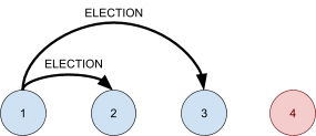
	Process 4 fails and 1 reacts by sending ELECTION messages to all processes with a higher ID.
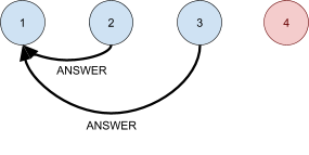
	Process 2 and 3 answer process 1’s ELECTION message.
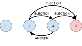
	Since processes 2 and 3 received ELECTION messages, they themselves start elections too. 3 answers 2, so 2 waits for a COORDINATOR message from someone higher up. 3 doesn’t get anything back from process 4 because it’s failed. 3 is about to hit the timeout and declare itself the coordinator, until...
	Uh oh! A rat is going to nibble on 3’s cabling and shut it down! 3, look out! He’s got air pods on, he can’t hear me! Oh god oh fuck I’m literally crying and shaking right now
	Oh no! Process 3 goes down before it can declare itself as the coordinator!
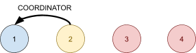
	Now 2 is waiting for a COORDINATOR message, but it’s not going to get one. 2 reaches the timeout and declares itself as the coordinator! It sends the COORDINATOR message to all participants below itself.
	1 receives the COORDINATOR message and declares 2 the coordinator.

So, what’s good about this algorithm?
It doesn’t exactly have safety because even though lower process IDs yield to higher ID ones, if a failed process revives itself while some lower process ID is declaring itself the coordinator, you’re going to get two different coordinator messages flying around! Who are you going to believe?
It has liveness because all processes participate and know the coordinator at the end.

So what’s the performance like?

Best case

Worst case

When the coordinator is process N, and N fails, and N - 1 detects that failure and elects itself using COORDINATOR messages.

There’s only an overhead of N - 2 coordinator messages and a delay of 1 message (because there’s no ELECTION/ANSWER messages, only the COORDINATOR messages being passed to everyone)

When the least identifier process detects coordinator failure.

There’s a total overhead of (N + 1)(N - 2) messages. Basically, that’s an O(N2) complexity.

Plus, there’s a huge delay of all the election and answer messages swarming around.

Reliable and Ordered Multicast

Multicast is used for group communication
You spread one message amongst a group of participants
However, how do you ensure reliability (every process gets the message) or order (multicasts sent before should come first)?

We’ll come back to those in a second, but first, let’s set some ground rules.
Here are some basic operations:

multicast(g, m) sends message m to all members of group g
deliver(m) delivers the message m (think of it like an acknowledgement of receiving the message, or a callback. Basically we run this as a confirmation of “yes, we’ve got the message”)

Message m contains information about the sender and the destination group.
Closed vs open groups: only group members can multicast to a closed group, whereas non-members can multicast to an open group.

If you still don’t understand how deliver(m) works, think of it like this: when a node receives a message m, it won't actually "get" it until it runs deliver(m). Say if a node receives m1 and m2, but it receives m2 before m1, but it should've received them in order m1, and then m2. Some systems allow the node to wait until m1, and then run deliver(m1) and then deliver(m2). So you see, deliver is mainly used to order messages that were received in the wrong order.

Basic multicast

This is just your normal multicast. It doesn’t guarantee reliability or order.

It works like this:
When we do multicast, we send the message m to each process p in the group g.
When a process p receives message m, it delivers message m to p (acknowledges it)

It really is basic; it’s just sending the same message to all the processes in the group, which is what multicast is, really.
Also works for open groups!
Only thing is, like I said, it doesn’t guarantee reliability (i.e. it can’t handle process or omission failure) or order.

Reliable multicast

This version of multicast tolerates process crashes, so it guarantees reliability.
It assumes the following:

Group membership is known (it knows about everyone in the group)
Reliable communication
Processes only fail by crashing
Closed Group

It works like this:

Process p basic-multicasts to all members of a group g (including itself)
When a process receives a message, it performs basic-multicast again (unless we’re the original sender) and delivers (acknowledges) the message for itself.

So basically, when we receive a multicast message, we multicast the same message too.
Duplicate messages are identified and not delivered.
When receiving a duplicate message, processes do not deliver (acknowledge) the message twice.

Reliable multicast guarantees:

Integrity: a process delivers a message at most once and only group members receive it
Validity: processes deliver (acknowledge) their own multicast messages
Agreement: if a process delivers (acknowledges) a multicasted message, then all other processes should too (all or none)

This algorithm is good, but it’s inefficient and does not ensure order.

Ordered multicast

Ordered multicast ensures order (obviously).
However, there are different kinds of order:

FIFO order: if a single process multicasts message #1, and then message #2, then all receiving processes must deliver (acknowledge) #1, and then #2. Messages sent by different processes can come in any order, since they’re not related.
Causal order: like FIFO, except it incorporates things like response messages and the relation, so if , then m1 will be delivered first and then m2.
Total order: all processes receive messages in the same order (it doesn’t have to be the order in which they’re sent, just that all processes receive the same order of messages)

Causal order implies FIFO order, but total order does not imply FIFO / causal order (because total order says nothing about when the messages were actually sent)!
Here’s a visual example:

Type of order	Image	Explanation
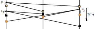
FIFO		In the diagram, messages are being sent between three processes. The blocks are the “receiving” events, and the small black circle dots are the “sending” events. The F1 message (beige blocks) is sent before the F2 message (black blocks) in the same process, hence why you’ll always see, in all processes, beige blocks before the black blocks. The F3 message (orangey brown blocks) is independent of the other messages, so the orangey brown blocks can go anywhere between the other blocks.
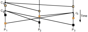
Causal		It’s clear that because C1 was sent before C2 in the same process, so the beige blocks will always go before the black blocks. In this example, let’s say that C3 is sent in response to C1 (the beige block), so is true and the orangey brown blocks will always go after the beige blocks. However, C2 and C3 are independent of each other (concurrent), so black blocks and orangey brown blocks can go before or after each other.
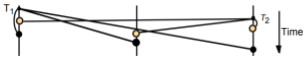
Total		It doesn’t matter when the messages were sent, each process has the same order of receiving messages: beige, then black.

So now we know the different flavours of ordered multicasting; what do they actually do?
It’s not important to know the details, just a rough idea is enough.

With Ordered Multicast: FIFO Ordering, sequence numbers are used.
All processes keep a counter of how many multicast messages they’ve sent.
They also package their messages with this counter too.
The counter is incremented when a message is sent.
Processes remember the latest sequence number of the latest message that they received from each process from their group (by default, they probably start at 0)
Messages sent out of order will be queued until the previous messages have been delivered (this is done using the counter in the message).
For example, if process P2 collects message #2 from P1 before it receives message #1, it’ll know to wait for #1 first before delivering #2.
This works with basic / reliable multicast.

With Ordered Multicast: Causal Ordering, we assume that groups are closed and non-overlapping.
We need to use vector timestamps. Don’t be afraid! It’s pretty much the same use as in the “Time in Distributed Systems” topic.
Each process has their own vector clock, starting at (0, 0, 0 .. ).
When a process sends a message, they increment their slot (e.g. P1 may increment to (1, 0, 0 ...)) and include their vector clock in the message.
When a process receives a message, it does one of two things:

If we haven’t got the messages that causally precede this message, put it in a queue.
If we have the messages that causally precede this message, then deliver (acknowledge) it and check the queue for messages that come after this one (and deliver those, too).

Don’t think about how the vector clocks work too hard; just keep in mind that, with the vector clocks, you can tell if a message causally precedes another message.

If you’re still confused, take a look at this example diagram which should clear things up:

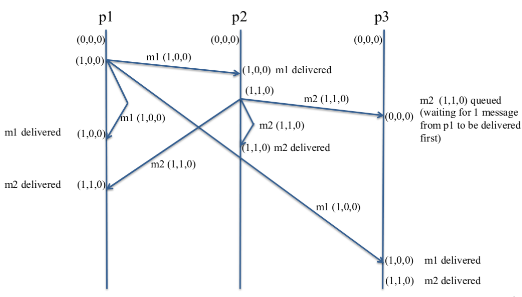
With Ordered Multicast: Total Ordering, we use group-specific sequence numbers.
This is like FIFO, but instead of the counters being specific to each process, it’s specific to the whole group.
For example, when process P2 collects message #2 from P1, that’s not 2 as in “the second message that P1 sent”, that’s 2 as in “the second message that everyone in the group has sent”.
However, to manage something like this, you’d need either a:

sequencer process to assign sequence numbers (then you’d need an election)
distributed agreement on the assignment of sequence numbers

It’s actually impossible to implement total ordering multicast in an asynchronous system, because doing so would mean we can have complete consensus in an asynchronous system, which is impossible.
Think of consensus as being reducible to total ordering multicast (you know, like with Turing machines).
More info on that in the Consensus topic (hype)!

Consensus

What is consensus?
Consensus is simply a network collectively picking an option over a set of options, after one process proposes a value.
Let’s look at an example:

Kris, Ralsei and Susie need to agree on either defeating King or not (to spare Lancer’s feelings, you see), but can only talk to one person at a time.
However, there is a twist! Toby Fox changed the plot, and now Ralsei is a secret agent working against our Lightner heroes! He’s planning to mess up our arrangements by giving us false information!
Is there some protocol they can use to decide, despite our traitorous friend?

To solve this means to solve our consensus problem.

The consensus problem can be applied to more than just Deltarune fan-fictions:

Banking: should we commit or abort transaction?
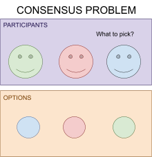
Replicated data: should we commit or abort updates?
Agree on message delivery order in total order multicast (more on their relationship later)

We also need to reach a verdict despite arbitrary process failures!

First of all, we need some assumptions:

There are N processes
We have a reliable connection (messages are always received)
Must tolerate both crash failures (someone drops out) or Byzantine failures (someone lies, like our prince Ralsei)

So how do we actually reach consensus? What’s the algorithm for it?
First:

Processes are all in an undecided state
Each proposes an initial value drawn from the set of options

Then:

Everyone exchanges values with each other (using reliable multicast)
Each process decides on a value and enters a decided state

Basically, if you’ve done the second coursework for this module, you’ve implemented this already.
You may be thinking “So what’s the problem? This looks fine to me.”
The problem is, does this still work when people start lying, or crashing?

Here are some properties of consensus that we want to achieve:

Termination: eventually, each process comes to a conclusion
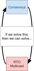
Agreement: all processes agree on the same option
Integrity: if all processes propose the same value, then all processes must agree on that value at the end too (basically, no changing your mind!)

So if the algorithm has no failures, how does it fare?
It has termination and integrity because it uses reliable multicast
Because it’s a majority vote, we have agreement
But with failures, it doesn’t work so well anymore!

With crash failures, asynchronous systems can’t detect that (doesn’t know if they’ve crashed or if they’re just really slow)
With Byzantine failures (lying), you need a certain number of truthful participants (this is even hard for synchronous systems, let alone asynchronous)

Now just before we jump right in to how synchronous and asynchronous differ, let me tell you what’s so special about consensus and RTO (reliable total order multicast).
This is assuming that only crash failures are allowed!
It can be said that if we solve the consensus problem, we can solve the RTO multicast problem.
If you’d like, you can think of it like consensus is reducible to RTO multicast, except it works both ways.

Implementing consensus using RTO-multicast:
Processes pick their options
Everyone uses RTO-multicast to multicast their options to everyone
Everyone picks an agreed option based on message order (last option, first option, whatever. It’s usually the first option)
Boom; you’ve got a consensus.
This works because to do RTO-multicast, the participants have to have a consensus on the order of messages, so we can just use that to our advantage.

Implementing RTO-multicast using consensus:
For each value to be delivered, run a consensus algorithm to distribute it to everyone.
Because the consensus algorithm picks one option out of many, for each run you do, the outcome of that consensus defines the order of the RTO-multicast.
For example, if the first run they decide on A, then the second run they decide on C, then the third run they decide on B, the consensus algorithm has pretty much mapped out a global order for us: A, C, B!

Synchronous

If processes crash, then we need rounds to make the algorithm work.
In all these rounds, participants send new votes to each other.
This works because even if a process crashes, as long as it sends its vote to one other participant, that participant will send that new vote to other participants, and soon everyone will know that vote, long after that participant is dead!
At the end of it all, everyone should have the same votes (because the rounds can only end if there are no more new votes to send)
Hence, everyone can decide on a vote.

If there’s no failures, we can just use 2PC (Two-phase commit). That works fine.
In fact, 2PC is literally just consensus, except the participants don’t share votes.
It’s like a non-failure-safe consensus!

What about arbitrary failures?
Ah, now here’s where it gets interesting.
Let’s say you have processes , and of them are liars.
Did you know that it’s impossible to get a consensus if ?
In other words, if a third of your participants are liars, there’s no way you can get a consensus. This is called the Byzantine generals problem.

Where did this rule come from?
Let’s go back to our example above:

Kris decides that they should defeat King.
Susie wants to hear everyone’s opinions. Kris says “Let’s defeat King”. Ralsei says “Kris doesn’t want to defeat King”.
What? They contradict each other! Who should Susie believe? Kris or Ralsei?
If only there was some other truth-teller that could be the tie-breaker in this dilemma...

In this example, and . , which is true, so no consensus can be made. If only we had one extra truth-teller, then we could reach a consensus.

Asynchronous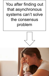

This is a bit of a depressing one (like the Halting problem)
Asynchronous systems don’t have timeouts, so we can’t tell the difference between a crashed process and a process that’s just taking its sweet time.
So there is actually no consensus algorithm for asynchronous systems.
If there is no consensus algorithm, that means it’s also impossible to solve RTO-multicast.

However, not all hope is lost. We can’t have a perfect consensus algorithm, but we can have an almost perfect algorithm using imperfect, close-to-reliable failure detectors.
In practice, this is usually good enough.

Consistency models

Don’t worry; SEC / CRDTs are not examinable, so these notes will cover standard models only. That means less reading for you!

So what is a consistency model?
Basically, it’s a network model that copies information between nodes.
Why do we want that?

Better performance
Better scalability
Better availability
Better fault tolerance

We go into more detail in Leonardo’s bit, but basically there’s this CAP theorem.
We can only have two of either:

Consistency: All nodes are updated with the right information
Availability: Requests are served as long as one server is available
Partition Tolerance: Stuff still works, even if we partition servers

There’s two main strategies we can apply:

Prioritise consistency (CP): high cost, no conflicts
Prioritise availability (AP): low cost, possible conflicts

We say there’s two strategies, but in reality there’s a range of models we can use.
At the top of the range, we have strong consistency models.

They use CP.
When updates are committed, replicas need a consensus on the ordering of the updates.

At the bottom of the range, we have weak consistency models.

They use AP.
No global ordering; guarantees on consistency are relaxed

So what are the kinds of models we can use?

Strong consistency (e.g. Google’s BigTable)
Sequential consistency
...
Causal consistency
Eventual consistency (e.g. Amazon’s Dynamo)

You need to learn all four of these, so let’s get started!

Strong consistency

Messages have global timestamps
The order of messages must respect these timestamps
Once a write is complete, all later reads return the value of that write or a later write.
Once a read is complete, all later reads return the value of that read or a later write.
So, for example, if process A writes something to a variable, and then process B writes another thing to that variable, the only thing people are ever going to read is that write that B did, because it overwrote A.
That’s it! It’s as you expect. Achieving this is expensive, and sometimes not necessary.

Sequential consistency

This one is a little weird. It may seem counterintuitive at first, but bear with me!
Sequential consistency takes the operations performed by all the nodes, merges them into a sequence, and operates that sequence.
Think of it like a card shuffle, but instead of cards, it’s operations.
I also have an example if it’s not clear:

We have nodes 1, 2, 3 and 4.
They each perform operations on a variable x, like so:

What sequential consistency does is, it takes all those operations:

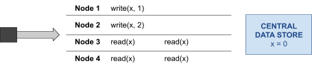
... and in each “iteration”, the arrow points to a node (it could be random, but it depends on the system), and it executes the operation on that “node queue”.
For example, let’s run the first iteration...

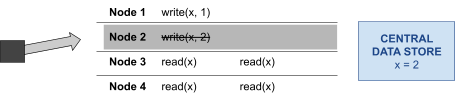
Look at that! The arrow picked node 2! So now the system executes write(x, 2) and writes x as 2 in the central data store...

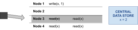
The arrow has now picked node 3, node 3 will read value ‘x’. It reads it as ‘2’.

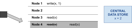
The arrow has now picked node 4, so now node 4 will read ‘x’ as 2.

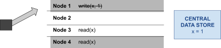
The arrow has picked node 1, so now x will be overwritten as 1.

... and then the arrow will pick node 3 to read, and then node 4 to read and then that’ll be that.

So, when you think about it, the arrow picked the operations in such a way that:

What? How can those reads at the end return 1, when just before read returned 2? How can reading something change the value?
It’s not that read changed the value of x. It’s that the write operation of setting x to 1 (from node 1) didn’t take effect until after nodes 3 and 4 read x for the first time.
Think of it like threads: let’s say node 1 was just really slow for some reason, and took ages to write 1 to x. By the time node 1 has a chance to do anything, node 2 has already written 2 to x, and nodes 3 and 4 have already read x as 2. But before 3 and 4 reads x again, node 1 changes x to 1, so when 3 and 4 reads x again, it’s 1.

The arrow in the example picks an order of operations, and those operations become global in the sense that all replicas will perform the operations in that order.
This is usually implemented using a totally-ordered multicast algorithm.
Shout out to James Bornholt for the analogy of using a “switch” to visualise sequential consistency in action!

Causal consistency

Causal consistency is a little stronger than eventual consistency, as it uses the event causality relation (if you forgot, it’s the a happened before b thing)
If it uses event causality, then yes, you guessed it, this uses vector clocks.
Again, don’t think about it too hard. Just keep in mind that, because of vector clocks, we can tell if an operation should go before another operation.
Because we use vector clocks, causal consistency has better performance than sequential consistency.

Basically, causal consistency makes sure that if , it’ll be sure to execute operation a before b.
If we have two concurrent actions, then we don’t really care; either way will do.

Let’s have a short example:

Now, if node 3’s first read(x) is a response to node 1’s write(x, 1), then when the replicas receive the operations to perform on their data, they’ll make sure to execute node 1’s write(x, 1) and then node 3’s read(x).
Assuming that all other operations are concurrent, it’ll do them in any order. Because they’ll do them in any order, causal consistency does not have a global order, making it less consistent than sequential or strong consistency.

Eventual consistency

Eventual consistency is lazy; it’ll eventually update the replicas.
But the implementation is easy; all you need to do is guarantee that updates actually reach the replicas!
However, we can have conflicts. If we do have conflicts, we can either:

use a consensus algorithm to decide, say, which write came first
roll back to previous configuration
delegate the problem to the application (let them handle it)

Amazon’s Dynamo uses the delegation solution to conflicts.

The main things about eventual consistency is that replicas eventually reach equivalent states, and that reads may not be up-to-date straight away.
The good thing is that the reads and writes are fast, because they happen in the background (they’re not such a huge priority), and this can work even if the network is partitioned.
The bad thing is that consistency is very weak and we still need consensus anyway for conflicts.

Garfield: Eventual consistency in cat form

Strong eventual consistency

I know you don’t have to learn this, but it’s just one sentence.
There’s a good compromise between all of these models; it’s called strong eventual consistency.
That’s all. Have fun with Leonardo’s section!

Other stuff (Leonardo)

Data Replication and Scalability

Data Replication

We can replicate data on multiple servers.
Why do that?

Fault tolerance: if one server crashes, the other one can still serve requests
Load balancing: we can distribute the pressure of requests
Location: we can place servers near users and increase performance

However, if we repeat data, how do we keep all the data on all the servers the same?
How do we achieve consistency?
Also, we want our service to be available if there is at least one server that’s up.
How do we achieve availability?

Primary-backup

This is one design choice that allows consistency and availability.
There is one primary server and multiple backup servers (linked through a master-slave pattern)
It works like this:

A client sends a request to the primary server.
If the primary server has already executed this request before, we go to step 5.
Primary server executes request and stores response
If it’s a write request, primary server updates and notifies all the backup (slave) servers and waits for ACKs (acknowledgements).
Primary server sends response to client.

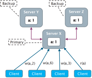
So basically, we have a main server receiving all the requests, and backup servers that are just updated with new information on the fly.

What happens when a backup server fails?
Easy; if a backup fails, it’ll eventually be restored / replaced, and then it’ll update its state from one of the other backups (if there is one), so we don’t overload the primary.

When the primary fails...

... how do we pick a new primary?
We can use an election algorithm to pick someone as a primary.
Since we need elections, and elections solve consensus, and it’s impossible to have a consensus algorithm in an asynchronous system, we know that primary-backup networks need to be synchronous! I just thought I’d tell you that.

... how do clients know who the new primary is?
The primary can register itself as the primary with a name service that clients consult.
Basically, there’s some service that the client asks “who’s the primary?” and the service goes “that guy”. The new primary can tell that service “hey, I’m the new primary now”.

... what happens to pending requests?
Clients resend the requests after a certain timeout, if they don’t get their response.
If the previous primary already executed and propagated that request, then we’ll just go to step 2 and respond.
If not, then we just execute the request as normal with the new primary.

How many server failures can be tolerated?
With N servers, up to N - 1 server failures can be tolerated (because we always need at least 1 server up)

CAP theorem

If you’ve read the previous sections, you already know what the CAP theorem is, but I’ll go into a bit more detail here:

Consistency:

All replicas are synchronised to have the same state
There must exist a total order of operations that is applied to all replicas (e.g. one guy can’t do operations in the order A B C and another do A C B, everyone has to do it in the same order)
If a read operation happens after a write, that read operation has to return the value in that write (which may seem trivial, but if you remember from consistency models, this isn’t always the case)

Availability:

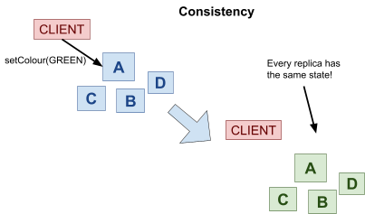
Requests are served as long as at least 1 server is up
Every request received by a non-failing node must result in a response

Partition tolerance:

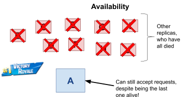
The data store keeps working if the servers are partitioned
In other words, the system needs to keep functioning even if two nodes lose communications with each other
Let’s say we got nodes A and B. They’re synced with each other and everything’s dandy. But, oh no! Here comes Gennaro with his rifle, and he accidentally shoots the communication cable between A and B while aiming for a fly! If we have partition tolerance, our system can still work and execute requests, even with A and B being independent from each other.

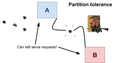
It’s impossible to have all 3, we can only have at most 2.
Why? Here is a short proof by contradiction.

Proof why CAP theorem is true
Let’s say all three are true; we have consistency, availability and partition tolerance.
Plus, we have nodes A and B, and a data value x = 0 initially.
We’ve got one client who can write to x and read x.
A and B are independent, and our system still works because we have partition tolerance.
Now, our client will write x = 2 to our node A (and A will acknowledge):

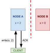
A can’t tell B about this write, because they’re independent.
Now the client will read x from node B:

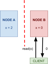
Uh oh! The client has read ‘0’ instead of ‘2’.
This breaks our rule of consistency, because as we’ve said before, if a read occurs after a write, that read has to return the value of that write.
As you can see, if we have all three rules, we’ve got problems.
However, we can have two out of three. Let’s have a look at those:

AP (availability, partition tolerance) systems
We give up consistency to always be available and to partition our system.
So, basically, it’s exactly like our proof above.
Is there anything close to consistency that AP can provide?
Well, there is partially synchronous networks, where we’re synchronous in “periods”, and asynchronous every other time.
So our nodes will eventually become consistent.
Eventual consistency is a good example of this.

CP (consistency, partition tolerance) systems
We give up availability to have consistency and partition tolerance.
When our nodes lose connection with each other, we respond to requests with a “FAIL” message until they’re back together.
So in that proof above, instead of writing 2 to x, or returning a ‘0’ when asking for the data value x, A and B would’ve just said “FAIL”.

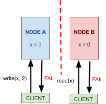
CA (consistency, availability) systems
This one’s a weird one, because here, we don’t have partition tolerance.
This means we don’t “support” partition tolerance.
It doesn’t mean we continue working when nodes are separated, or we fail when nodes are separated. It means our system is built such that the concept of “separating nodes” doesn’t exist.
This is only applicable to single-site systems (like datacenters) which are not likely to experience network partitions.
But if we have a single-site system, that defeats the purpose of thinking about data replication!
In a distributed system, you cannot give up partition tolerance: https://codahale.com/you-cant-sacrifice-partition-tolerance/
So CA isn’t really an option. We mainly care about choosing either consistency (CP) or availability (AP).

Scalability

What is scalability?
Scalability: the ability to handle increased workload without adding resources to a system, or to handle increased workload by repeatedly applying a cost-effective strategy for extending a system’s capacity.
Basically, it means your system can handle lots of work at one time.

How do we assess scalability?
There are three steps:

Scale parameters: the external parameters that change over time, the things that affect scalability (number of clients, workload, number of data objects etc.)
Scalability metrics: stats and measurements of system properties based on parameters

Latency: how long it takes to complete requests from POV of clients
Throughput: how many requests per second are processed
Availability: probability that a system will work currently during a certain period

Scalability criteria: expected scalability metric values (where your metrics should be at. You wanna hit as many of these as you can)

Worst latency observed by 1% of requests
Four nines availability: be available 99.99% of the time

Sounds amazing but it’s still around 53 minutes downtime per year

It’s always cool to add stuff to your system to make it more scalable, but...
... there’s a point at which adding stuff doesn’t give you enough benefit to make it worthwhile.
This is called the law of diminishing returns.
The more servers you add, the more scalable your network is, right?
But what if you had 9,357,572 servers, and you added one to make it 9,357,573? Would that make much of a difference?
Probably not. You need to strategize your scalability tactics to be more effective!

One good scalability tactic is to identify bottlenecks and mitigate them.
For example, in the primary-backup model, there are two bottlenecks:

The primary server, as it’s the one handling all the requests
The backup servers, as the primary needs to wait for all the ACK signals

Here’s what we can do to mitigate them:

Share data on more than one primary server
Primary server only waits for majority of ACK signals

But here’s the drawbacks:

If there are data dependencies, we’ll need coordination amongst primary servers
Not all backup servers might be up to date, and if the primary fails and a backup server is elected that isn’t up to date yet, we’ll have problems

Is it worth the risk? I don’t know. I just write the notes.

Highly Available Distributed Data Stores (Amazon Dynamo)

What is Amazon Dynamo?
How does Amazon Dynamo work? it just works
It’s a distributed key-value storage service run by Amazon.

Key-value store means that data are stored such that each value is mapped to a key, like how a map data structure works

It’s used for things like:

Shopping carts
Best seller list
Customer preferences
Product catalogue

Now, before you begin, keep this in mind: in the exam, it’s not important to know the intricate details! So if you don’t exactly understand how something works, don’t worry too much. You’ll probably be asked things like “How well does Dynamo scale?” or “How is Dynamo an AP system?”, not something like “When you have a ring in Dynamo and you get some data and nodes A, B and C are down and N = 10 and W = 5 and R = 4 and lalalalalalalalalalathequestiongoesonforever” so be sure you understand the concepts of Dynamo, and don’t sweat it if you don’t understand the underlying mechanics too much.
This applies to every other system in Distributed Systems & Networks.

Replication

Amazon Dynamo has the following interface:

get(key)
put(key, context, object)

It seems like something you’d expect for a key-value structure, except the context object.
We’ll go over that more in detail later, but it’s basically for specifying the version of the object to update.

So what kind of structure is Amazon Dynamo?
It uses a Distributed Hash Table (DHT), but with a slight adjustment.
Basically, we have a ring of nodes:

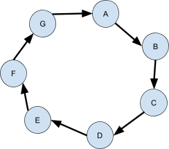
When we put a key-value pairing (e.g. K -> O), we hash the key and it gets a respective position on the ring for that key (think of it like the wheel of fortune; the key points to a “random” (it’s based on hash) spot on the ring):

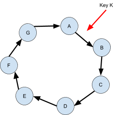
Now, that data object (key-value mapping) is replicated on at least N nodes, from that position, clockwise (say that N = 3, but we decide to replicate 5):

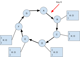
Those 5 nodes make up K’s preference list, which is a list of nodes that is responsible for a certain key.
Each node is responsible for the keys between itself and its Nth predecessor (e.g. D is responsible for keys whose position lie between itself, D, and it’s Nth predecessor, A, because any keys that fall in that range will be added to node D)
The reason why we pick more than N nodes is to account for node failure, so if one of the first N nodes dies (B, C or D), we can use the other nodes (E or F).

Consistency

Dynamo sacrifices consistency for availability, but it can have conflicts.
It ensures consistency by allowing changes to propagate to other nodes in the background over time, making Dynamo a lot like eventual consistency.

How does Dynamo resolve conflicts?
It resolves them at read time, so when you try to read data, that’s when the conflict is resolved.
First, Dynamo tries to do it by itself using distinct data versions (using vector clocks), but if it has trouble, it’ll send the client the list of versions.

How does Dynamo’s get / put requests work?
First, Dynamo finds the first node in the preference list for that key, which becomes the request coordinator.
A request invokes the get / put operation on the first N healthy nodes in the preference list (including the request coordinator).
Now here is where it gets complicated:
Two numbers are picked, W and R.
W is the minimum number of nodes that must perform the put request
R is the minimum number of nodes that must perform the get request
When doing a put request:

Request coordinator performs put locally, then sends the new version to the other N - 1 nodes.
Once the request coordinator gets W - 1 responses, then the write is successful

When doing a get request:

Request coordinator asks all other N - 1 nodes.
Once the request coordinator gets R - 1 responses, then the read is successful. If different versions are found, we return all those that are causally unrelated (concurrent) (basically, a byproduct of syntactic reconciliation).

So, basically, when we write, W out of N nodes are updated, and when we read we consider R out of N nodes’ read operations.
Which nodes out of N are picked? The ones that respond first, usually.

There are several combinations we can get out of this:

- can return stale versions of the object

Image

Explanation

Here, we’re putting K = 2 into their respective nodes. Since W = 2, we’ll only accept 2 node responses. The green nodes are the nodes that have sent write responses first, filling up our W window.

For some reason, the request does not reach D, E and F.

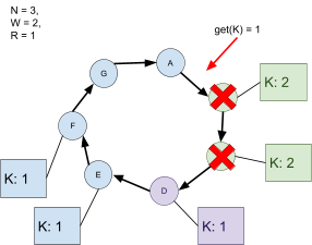
Here, we’re trying to get K. However, node D responds because B and C are down. Now we’ve got a stale version of K!

- when we read, we can get multiple versions, leading to a quorum-like system

Image	Explanation
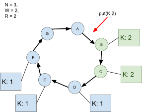
	Like last time, we’re putting K = 2 into their respective nodes. Since W = 2, we’ll only write to the 2 most available nodes. The green nodes are the nodes that have written the update.
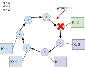
	Here, we’re trying to get K. B goes down, and R = 2, so we’ll fetch the values C and D have. They’re two different versions: one is old and one is new!

- optimise reading (because only one node is doing it)
- optimise writing (because only one node is doing it)

When R = 1 or W = 1, it’s quicker, but we have less consistency.
For better latency, R and W are usually configured to be less than N.

There’s a problem with this, though!
A put operation may return before all the nodes are updated, so get operations may return outdated objects.

How do we fix this?
We use versioning!
Basically, if we try to update an object that hasn’t finished updating yet, we create a branch, similar to Git.
We need to diverge the branches; we don’t want to deal with lots of branches!
There’s two ways to diverge them:

Syntactic reconciliation
If the new version subsumes the previous version, then reconciliation is easy.

Semantic reconciliation
If there’s a bigger conflict, then we will send the branches to the client and the client will take care of it.
For example, with a shopping cart, we would union the carts; the data from adding to a cart is never lost but deleted cart items may resurface
With each version of the object, a vector clock is attached.
The vector clock slots consist of a pair, containing the node ID and the update count.
The context object we talked about before contains vector clock information.
When we send branches to the client, we also send their vector clock information.

Can we see this in action? Of course we can!

Image	Description
	Here, we write Object #1, written as O1, by node Sx. This is the first time Sx has written anything, so it gets the value of ‘1’ in its vector clock spot.
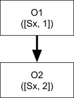
	Here, we overwrite the object with #2, also done by node Sx. As a result, the update count for Sx is now 2.
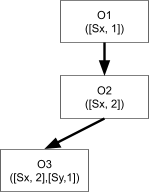
	We write yet again, to object #3. This time, node Sy does it, so Sx’s counter stays at 2, and Sy’s counter becomes 1.
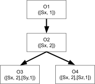
	Here’s where things get interesting though: Sy’s writes are taking a long time. Maybe there’s lag. Anyway, the client overwrites with #4 and Sz, a new node, writes that. Now, a new branch has been formed, because there were two changes to the same version, #2.
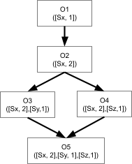
	Now we’re doing a new read. The client finds out that there’s a conflict and there’s branches to join together. The client fixes the conflict and pushes object #5. The vector clock still takes into account who has updated the object in all branches.

Fault tolerance

How does Dynamo handle faults?
It uses something called sloppy quorum.( ͡° ͜ʖ ͡°)

Basically, if A temporarily goes down, and we want to do some put request, we’ll send the update to D, and D will do the put request instead.
The reason why we don’t send it to B or C is because B becomes the new coordinator, hence B and C would know of the operation.
Then, when A is back online, D will tell A about the update.
The update has a hint in its metadata that suggests which node was the intended recipient, so D is able to know to inform A of the update.

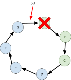
This is called hinted handoff.
This way, Dynamo ensures that get/put requests do not fail due to node/network failures.
Additionally, we can achieve the highest level of availability if we set W to 1, since we only need one node to be available to write anything.

Dynamo also has something called replica synchronisation, where a periodic protocol runs in the background and ensures data is synchronised between nodes.
It’s based on Merkle trees.
It solves the problem of node D failing before it can update node A in hinted handoff.

Why is Amazon Dynamo AP?

Sloppy quorum allows Dynamo to serve even when nodes go offline
Additionally, there are consistency conflicts, so it’s definitely not CP.
They’re resolved through:

Syntactic / semantic reconciliation
Replica synchronisation

So eventually all replicas will converge, which means it follows eventual consistency.

Scalability

Since the keys are dotted around the ring when hashed, data is distributed amongst the nodes pretty well.
It’s also really easy to add nodes to the ring!
Let’s show an example:

Remember our first example?
N is 3, so B is in charge of keys landing anywhere between F and B.
C is in charge of keys between G and C.
D is in charge of keys between A and D.
What if we add a node X between A and B?

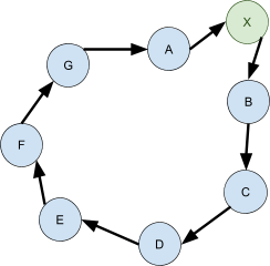
B isn’t in charge of F to B keys anymore; it’s in charge of G to B, because X has distanced B away from F!
C is now in charge of A to C
D is now in charge of X to D
Since B is no longer in charge of any keys between F to G, B can send all those keys to X, because X is now in charge of them.
Additionally, C will send all keys from G to A to X...
... and D will send all keys from A to X to X.

That’s it! Now everything is stable again.
Dynamo is scalable; the more nodes you add, the less keys each node has to remember.

Consistent Distributed Data Stores (Google BigTable)

BigTable, like Amazon Dynamo, is a service that Google provides that stores data.
Google uses it themselves, for things like Google Earth and Google Finance.

Data model

BigTable fulfils five properties:

Sparse: NULL values aren’t stored, to save space
Distributed: data is distributed amongst nodes
Persistent: data is saved on stable storage
Multi-dimensional: data is indexed by row, column and timestamp
Sorted: data is stored on disk in some defined order

So how does BigTable actually work?
Well, you know tables, right? I hope you know what a table is.

ID	Name	Part	Stand
1	Jotaro Kujo	3	Star Platinum
2	Josuke Higashikata	4	Crazy Diamond
3	Giorno Giovanna	5	Gold Experience

Well, in BigTable, categories are clumped together, so instead of accessing a row with all its columns, you can specify a row with a column family, containing columns that are often requested together.
For example, let’s say Name and Part are clumped together in a family.
We could specify any row, and the family, and we would get back data sets like:

1 : “Jotaro Kujo”, 3
2 : “Josuke Higashikata”, 4
3 : “Giorno Giovanna”, 5

Each cell can be timestamped, so if cells change, different versions are created and timestamped.
There’s also a garbage collection scheme to either keep only N versions available, or to delete versions past a certain date.

There’s also an implementation of BigTable called WebTable, which Google uses to handle webpages.

The row (ID) is the URL of the webpage.
The columns are the properties of the pages (content, links, language etc.)
The cells are timestamped when the information is retrieved

There’s also an anchor column family, which stores references to the page (think Google PageRank).

Architecture

Rows of column families are stored in tablets, sorted by key.
A tablet is like a storage unit that contains some rows.
A bunch of tablets are stored by a tablet server.
All the tablet servers are managed by a master server.
Clients directly talk to the tablet servers and the master server.
Clients ask the master server what tablets to talk to in which server, and the client reads/writes data through the tablets in the tablet servers.

Caution: The data isn’t actually stored in the tablet! It points to the SSTables (files, see below), with the corresponding data, within the GFS chunkservers (also see below).
The data is only stored in the tablet from a logical perspective, but the chunkservers of GFS are where the data really resides.

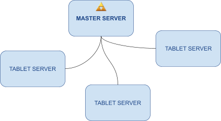
BigTable has a file system, called GFS (Google File System).
Files are divided into fixed-size chunks (of around 64MB), kind of like sectors on a disc.
Chunks are replicated on multiple chunkservers (around 3).
The master from before manages all the chunkservers, and stores things like:

Namespace (to help navigate the chunkservers)
Access control information
Mapping from files -> chunks
Mapping from chunks -> chunkservers

Clients ask the master what chunkserver it should talk to, and then the client talks to them (the client being BigTable; actual clients don’t talk to the GFS system)
The master can also cache queries by the client.

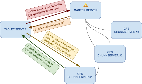
There is one more unit called chubby. It’s highly available.
Chubby is like a configuration server that stores all the useful tidbits and parameters that BigTable requires to function, such as:

Persistent concurrency locks for files and directories
Handle tablet server lifetimes
Store schema information
Ensures that there is at most one active master at any time

It contains a small namespace with files and directories, and reads/writes to files are atomic.

The entire architecture looks like this:

What about scalability?
What happens when there are more client requests?
Tablet servers receive more traffic, because clients directly talk to them. With more traffic to tablet servers, tablet servers are requesting the chuckservers more, so the traffic of tablet servers are proportional to the traffic of chunkservers.
The master server only has as much traffic as there are clients who need to know what tablet servers to talk to; they’re not as often spoken to as other servers, like tablet servers or chunkservers, so they experience less traffic.

What is the bottleneck?
Tablet servers and GFS chunkservers, because they’re the ones that all the clients are requesting writes / reads from.

What can be done to mitigate the bottleneck?
You can add more tablet servers / chunkservers, so the data is distributed more and there is less stress on individual servers.
However, the more tablet / chunk servers you have, the closer their strain gets to the master’s strain. Sooner or later, the master’s strain will be higher than the tablet / chunk servers’ strain. If that happens, the master itself will become the bottleneck! Plus, it doesn’t help that there are more servers to request about from the master.

Tablets

There are multiple levels of tablets:

First level: Chubby points to root tablet
Second level: Root tablet points to METADATA tablets
Third level: METADATA tablets point to user data tablets

The client library caches tablet locations and also prefetches locations of tablets the user might want to use next.

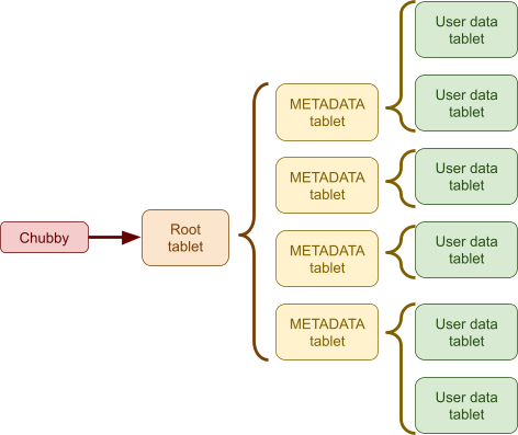
The master server can keep track of:

Mapping from tablets to tablet servers
Unassigned tablets

The master has a unique “master lock” in chubby.
If the chubby session expires, the master kills itself.
If the master dies, a new one is promptly started.
When there is no master, client requests cannot be served.

When a tablet server starts, it acquires a lock in chubby, in the form of a file in some server directory.
The master monitors this server directory to discover new tablet servers.
The master detects if a tablet server isn’t working by:

Asking the tablet server about its lock
If there is a problem, the master tries to get the server’s lock itself
If the master can get the lock, that means the chubby is OK, it’s the tablet server that’s the problem
When the tablet server has a problem, the master deletes all the chubby files associated with it and moves the associated tablets to the unassigned tablets.

If a tablet server loses its lock, it stops serving requests. It’ll try to acquire its lock again as long as the file exists, but if the file does not exist, the server will kill itself.

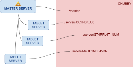
SSTables

An SSTable (Sorted Strings Table) is a file format used by BigTable to store information.
It is a persistent, immutable ordered map from keys to values.
Remember, it’s immutable, so we write once and we only read from it afterwards.
We can either look up a single key or iterate over multiple key-value pairs in a key range.
It’s also split up into blocks, and we can use a block index (which is at the end of an SSTable) to search for blocks and load them in memory.

So what happens when we write to a tablet?
The write operation goes into a buffer called “memtable”.
As we request more write operations, more goes into the “memtable” buffer.
Older updates are stored in the SSTables.
The writes are also logged into a commit log.
The read operation is done by merging the memtable and all the SSTables together to get a single value.

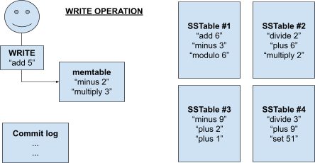
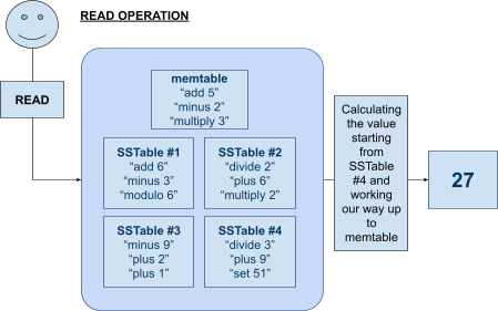
So what happens to the operations in the memtable? How do we create new SSTables?
We have something called minor compaction, where we empty out the memtable into a new SSTable.
We also have something called major compaction, where we compress all the SSTables and the memtable into one big SSTable (like merging layers in Photoshop), so that we don’t end up with thousands of SSTables.

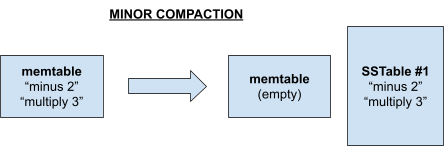
Why is Google BigTable CP?

Availability is given up in the following situations:

If the master dies, no requests can be attended to
When a tablet server dies, the tablets that were handled by that server cannot be used until they are reassigned
If chubby fails, no synchronisation or client requests
If GFS fails, SSTables and commit logs cannot be accessed

Consistency exists in the following situations:

Each row is managed by a single tablet server (requests are serialised)
Writes for a specific tablet to GFS are done by one tablet (reads and writes are serialised)
Writes to GFS are always appends (copy-on-write), so concurrently there are no race conditions (because data is immutable, for more info check PLC notes)
SSTables are write once and then read, so there’s no interleaving between reads and writes
Commit logs are only read upon compactions and recoveries; reads are not interleaved with writes

Therefore we have strong consistency.

Online Distributed Processing

How do we process streams of data / event-based data online?
Our process can’t quit, because data streams are continuous.
There exists services to help us process data like that!

Use cases

It’s used by Twitter to look at trends coming and fading. That can be interpreted as a data stream, and trends are happening all the time, so the system has to always be on, running and parsing data.
It can also be used by Google Trends for search queries.
It’s also used for user profiling, bus routing, sentiment analysis in tweet streams and fraud monitoring.

Requirements

So what do we actually need?
We need:

Real-time computing
Low computation latency (do stuff fast)
Correlation with fresh data (don’t use old stuff)
Input loads can vary (be scalable)
Hardware / software failures may occur (be fault tolerant)

Apache Storm

Apache Storm is an implementation of this.
It has an abstraction that can work with event-based data, it can sustain high input streams and can parallelise computation.

Data model

So how does it actually work?
It works like this:

Spout: outputs the raw data that we want to work on
Bolt: modifies the data in some way and either passes it on to another bolt, or stores it

The topology usually looks something like this:

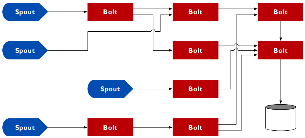
For example, if we wanted to implement some word counting example, we could have:

One spout for the raw data string
A bolt to split the string into words
Another bolt to count the words

So we have something like:

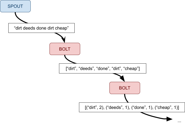
Architecture

So that’s the high-level stuff, what about the low-level stuff?
A storm cluster (one of the things we have above) consists of one master node and several worker nodes.
The master node runs the Nimbus process, which manages all the workers.
The worker nodes run Supervisor processes, as well as a number of worker processes.

The topology is submitted to the master, and the master allocates a component for each Worker node using a scheduler.
Each component can have multiple instances, and each instance is mapped to an executor (a thread).
Workers (processes) are run when the Worker node must run executors for the given topology.
Each Worker node handles their own local input / output, and the supervisor makes sure everything is running alright.
The Nimbus handles potential failures and resource usage.

Replication

Let’s say you have a stream of integers and you wanted to use this architecture to perform some operations on it:

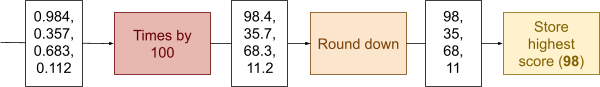
The yellow operation is stateful, because it requires a state to run (it needs to remember the previously highest score)
The red and orange operations are stateless; they are pure functions and do not rely on some kind of memory or state.
Therefore, we can split the data we receive and replicate these stateless functions to create a pipeline:

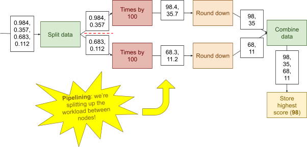
We can replicate the same list of stateless operations as many times as we want (within reason). The number of times we do this is called the replication factor.
We can apply this practice to Apache Storm, with spouts and bolts:

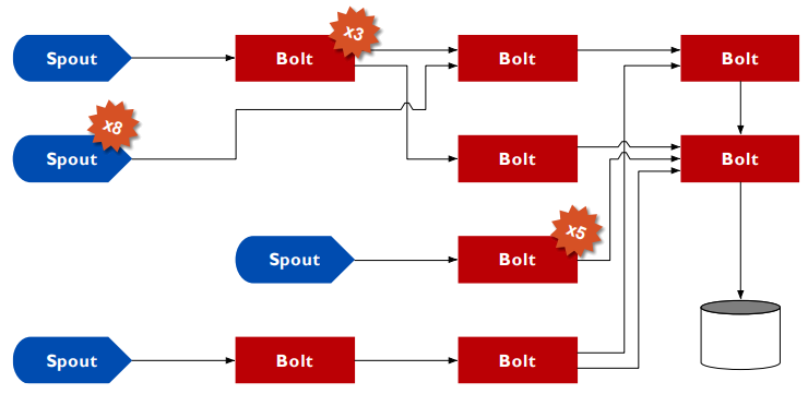
When we have multiple spouts (like that Spout x8), nodes won’t be so clogged with input data; it’ll be distributed, so even if we receive an influx of data, our system won’t crash.
When we have multiple bolts (like the Bolt x3, or the Bolt x5), we are doing the same thing as the example above; we’re pipelining stateless operations to split up the workload amongst multiple nodes.

Stream grouping

But how do we split up the data to distribute? In the example above, we just chopped the data in half and fed each pipeline half the data. In practice, that may not be the most efficient approach; we may be able to optimise our splitting by choosing the right grouping strategy!
Types of grouping strategies:

Shuffle: data is randomly distributed between pipelines
Fields: pipes data based on some predicate on their fields
All: all data is distributed on all pipelines (may be useful if randomness is involved)
None: you don’t care (by default, this is the same as shuffle, but in the future Apache Storm will change this)
Direct: the producer of the data directly picks a pipeline programmatically
Local or shuffle: will shuffle and pipe data only to the target nodes that are running on the same Worker node as the data source. If there are none that fit that description, then it just works like normal shuffle.

Sources: 1 2

These are Leo’s slides, so you know what we’ve got to do...
How does Apache Storm scale?
What happens when workload increases?
Computational stress increases for some spouts / bolts

What is the bottleneck?
The CPU or memory for overloaded spout / bolt instances

What can be done to mitigate the bottleneck?
Two things:

Increase the replication factor of overloaded spouts/bolts, so we distribute the workload
Add more Worker nodes so more systems can run more instances of the spouts/bolts, thereby distributing the workload

Fault tolerance

A tuple can spark the production of multiple tuples in the topology.
When we say tuple, we just mean some input data (it’s mainly to account for multiple data elements residing within one data unit)
What this means is that one piece of data going into the topology can result in a whole tree of resulting data units.

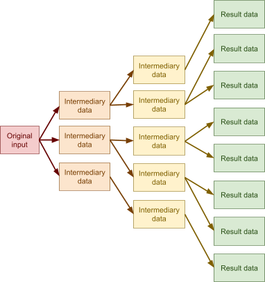
That looks like a mathematical structure...
That’s a DAG (directed acyclic graph)!

We have a component called an acker that monitors the DAG of each input tuple.
Each bolt sends an “ack” signal to the acker when they correctly process each input tuple.
When the acker receives this, it prunes the DAG at that bolt’s respective position.

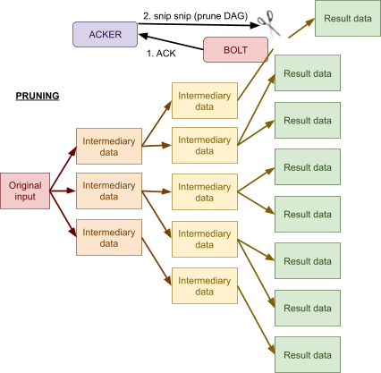
The acker goes along the bolts, from the finish to the start, receiving acks and pruning the DAG, until there’s nothing left of the DAG.
When the DAG is empty, the acker knows that the input tuple was processed correctly. In that case, the acker notifies the original spout of that input tuple for garbage collection.

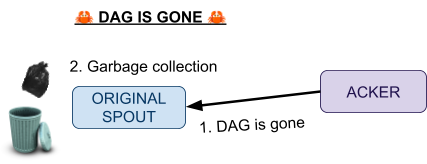
However, if there is a timeout and the DAG isn’t empty yet, the acker notifies the original spout about the failure and the spout will replay the failed tuple.

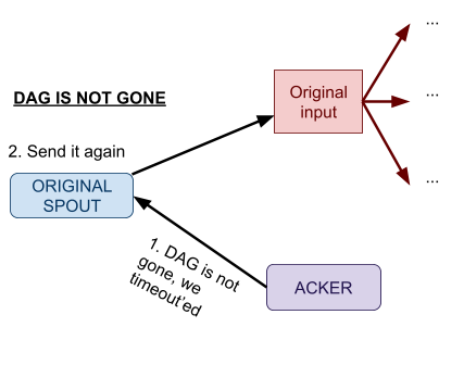
What about when spouts/bolts fail?
If a worker dies, the supervisor restarts it (unless it fails at boot time; then the Nimbus will reassign the work to a different machine).
If a machine fails, the assigned instances will timeout and the Nimbus will reassign them.
If the Nimbus/Supervisors die, they are restarted

They behave like a fail-fast process (better to die quickly than to waste time in a half-working state)
They are stateless in practice

There is no explicit state management for components in Storm.

Batch Distributed Processing

With online distributed processing, it’s highly complex and hard to maintain.
With batch distributed processing, incoming data is stored; not processed straight away.
It’s done in batches over time.
Therefore you can have a high input rate because it’s only being stored; it’s computationally less expensive than actually processing stuff.
However, because everything is stored, batch might not be suitable for real-time applications.

Implementation #1: Google MapReduce

Logically, computation is split into two phases:

Map: (k, v) -> list of (ki, vi)
Reduce: (k, list of vi) -> (k, v)

By doing this, we can simplify:

Parallelisation
Handling of machine failures

For example let’s do a word count example
Input: “Deer Bear River Car Car River Deer Car Bear”
Output: [(Bear, 2), (Car, 3), (Deer, 2), (River, 2)]
How do we do this with map and reduce?
It’s actually 4 steps:

Splitting: split input text into paragraphs (e.g. 3 words each)
Map: just map a word to the number 1
Shuffling: order the key-value mappings into groups of equal keys
Reduce: count the number of mappings and reduce to one key mapped to the count

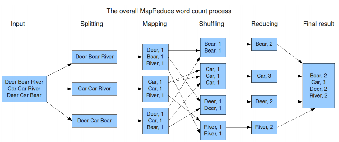
Implementation #2: Apache Hadoop

Hadoop also does map and reduce
However it has a job tracker, which delegates jobs to task trackers, which delegates tasks to task processes

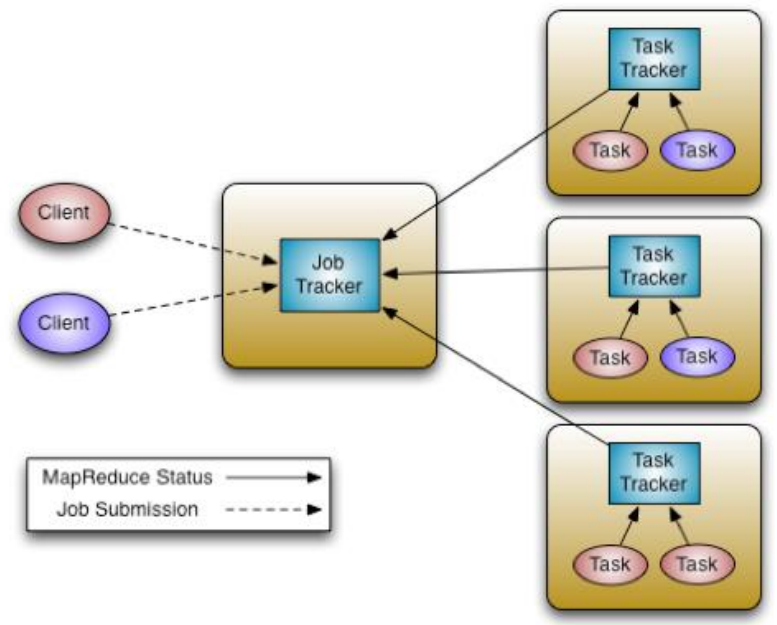
Task trackers have a limited number of tasks
If full, tasks go into a queue and wait for other tasks to finish
Bottleneck: if there're too many tasks and the task tracker can’t take them all, there will be too many tasks in the queue.
Solution: add more task trackers (seems simple enough)
If there’s too many task trackers, job tracker will become the bottleneck (unfortunately there’s no mitigation for that)

Hadoop Distributed File System (HDFS)
Remember GFS with BigTable? This is kind of like that.
Data is organised into files and directories.
It’s designed for:

Single writer
Multiple readers

Data is replicated for optimisation, minimising data loss and improving availability.

Data is divided into chunks, usually of max size 64MB (getting deja vu?)
Each chunk is replicated over DataNodes (chunkserver equivalent in BigTable)
The replication factor of DataNodes is a configuration parameter
The NameNode decides which chunk is stored in which DataNode.
When we write, access the NameNode first, and then write to the DataNote.
When we read, the NameNode picks out the closest DataNode for us.

What about splitting and shuffling that Google MapReduce had?
Yes, Hadoop does that too.
Each mapper keeps its own output partitioned by key and notifies the JobTracker about what keys it has.
Each reducer is informed by the JobTracker on what keys to process and collects the corresponding data from TaskTrackers.

Apache Hadoop has something called locality awareness.
In typical development, each TaskTracker is placed in a machine with its own DataNode.
Mappers get their data from DataNodes. Wouldn’t it be a pain if the mappers had to fetch data from nodes all over the network every time they wanted data?
That’s why the JobTracker assigns mappers to TaskTrackers with DataNodes storing data that the respective mapper needs.
When that happens, the mapper doesn’t need to fetch their data from across the network; they can just do it locally, saving lots of time and minimising data movement.

What happens when stuff fails?
If a task fails:

The JobTracker detects it
Task is assigned to another TaskTracker
If a task fails more than a certain number of times, the whole job fails
If a TaskTracker has too many failed tasks, it is blacklisted

If a TaskTracker fails:

It’s blacklisted (obviously)
All the tasks for that TaskTracker are reassigned to another TaskTracker

If a JobTracker fails:

It’s a single point of failure! (basically, you’re fucked)

TL;DR

Look! It’s the reference guide of Computer Science!
Well, more specifically, Software Engineering MEng...
How are you doing today? Good?
Studying hard?
What? No?
What’s that, you say? The slides are crap and make you want to commit not continue your lifespan any longer? You’re also too lazy to read the above notes because you’ve left revision to the last minute because you have no self-control and regret your life choices?
Scroll down. Don’t worry, I gotchu.
However, if you do have time, please read all of the above notes at least once before you move on to this reference section.

Kirk’s stuff

OSI model	TCP/IP model	Tanenbaum’s book
Application	Application	Application
Presentation	Transport	Transport
Session	Internet	Network
Transport	Link	Link
Network	Hardware	Physical
Data Link
Physical

Types of medium:

Coaxial cable
Twisted pair
Power line
Fibre optic
Wireless (laser, sound, ultrasonic, pulses, radar)

Packet: a unit of data in the Network layer (our payload)
Frame: a unit of data in the Link layer (what the link layer actually sends)

Hop by hop transmission: where data is transported through intermediate nodes to its destination.
Packet-switched network: A network where packets dynamically find their own way to a destination without a set path

Link layer models:

Connectionless, no acknowledgements
Acknowledged, connectionless service
Acknowledged, connection-oriented service

ARQ (automatic repeat-request): error-control mechanism that uses ACKs and timeouts to ensure reliable communications with unreliable recipient

Three kinds of ARQ protocols:

Stop-and-wait
Go-back-N
Selective-repeat

Detect errors using parity bit or CRC (cyclic redundancy check)

Ethernet: de facto link layer standard
Ethernet used to use CSMA/CD (Carrier Sense Multiple Access with Collision Detection)
Ethernet frames have priority setting from 1 to 7, which affects prioritisation at switches.
WiFi: wireless alternative to Ethernet. Works in 2.4GHz or 5GHz.
Wifi uses CSMA/CA (Carrier Sense Multiple Access with Collision Avoidance)
Can use Request to Send / Clear to Send (RTS/CTS) to increase performance

MAC (Media Access Control) address: a unique ID for network interface controllers (NICs) at the link layer. (48 bits long, can be extended to 64 bit)

Concentrator device: central hardware in a network; nodes connect to it

Hubs and repeaters: Old! Just reroute packets
Bridges and switches: Smart! Learn what packets go where

ARP (Address Resolution Protocol): a protocol used by host: given IP address, can get MAC address

4 kinds of message:

Unicast
Broadcast
Multicast
Anycast

IP address plan: range of local IPs a host can have
IP subnet: a localised network behind a router

Spanning tree protocol: enables and disables switches so a path is always available for packets (within reason)

VLAN (virtual LAN): a logical network; not physical. Each node can be in different physical LANs but be in the same VLAN.

IP (or Internet Protocol) is the main protocol used in the network layer.
Properties:

Packet-switched, connectionless
Unreliable
Routing
Globally unique, delegated addresses

Main protocols:

IPv4
IPv6
ICMP - for diagnostics and control
ICMPv6
IPSEC - for security

Store-and-forward packet switching: a technique where data is sent to an intermediary node, then passed on to either another intermediary node or the destination node. Basically the same as hop by hop transmission.

IPv4 datagram:

MTU (or Maximum Transmission Unit) is the size of the largest data unit that can be communicated in a single network layer transaction.
If data unit is bigger than MTU, fragmentation happens.

IPv4 classes:

Class	Prefix range	Prefix length
A	0.0.0.0 to 127.0.0.0	8 bits
B	128.0.0.0 to 191.255.0.0.	16 bits
C	192.0.0.0 to 223.255.255.0	24 bits
D	224.0.0.0 to 239.255.255.255	n/a
E	240.0.0.0 to 255.255.255.255	n/a

Maximise address space using:

DHCP (or Dynamic Host Configuration Protocol)
NAT (or Network Address Translation)
Classless Inter-Domain Routing

Properties of subnet:

Subnet network address
Subnet prefix length
Subnet mask (same information as prefix length)
Subnet IP broadcast address

Can use mask to get from IP in subnet to network address and broadcast address

ICMP (or Internet Control Message Protocol): protocol for checking status between hosts (pinging is included in this).
Router advertisement: telling other routers about yourself

Types of routing:

Static routing: configure routes manually
Dynamic routing: establish routes on-the-fly

Aggregating prefixes: sending packets to networks with smaller prefixes, so that we don’t need to access specific routers

Routers build up their routing table with routing protocols.
Distance vector: only talk to neighbouring routers and build up a shortest distance to our destination using the Bellman-Ford algorithm.
Link state: talk to all routers to establish full knowledge of site
Link state usually better than distance vector

Autonomous system (AS): a network or a collection of networks that are all managed and supervised by a single entity or organisation, typically an ISP (Internet Service Provider).

Interior routing protocol: exchanging routing information between gateways (routers) within autonomous systems
Exterior routing protocol: exchanging routing information between autonomous systems

Border Gateway Protocol (BGP): allowed autonomous systems to store and exchange routing information about packet destinations. The de facto exterior routing protocol.

UDP (User Datagram Protocol): connectionless, low overhead protocol; “fire and forget” basis
UDP properties:

Connectionless
Application layer has to retransmit, if required
Constant bit rate
Low overhead

TCP (Transmission Control Protocol): connection oriented protocol
TCP properties:

Connection management
Flow control
Tries to avoid congestion
Retransmission
Reassembles segments in correct order

TCP connection establishment:

	TCP	UDP
Connection	Connection oriented	Connectionless: “fire and forget”
Reliability	Handles ACK & retransmissions	Application needs to handle ACK & retransmissions if needed
Data Order	Guaranteed that it arrives and in the correct order	No guarantee that data is received in the order sent
Header	20-bytes minimum	8-bytes
Good for	Applications that need high reliability	Applications that need fast and efficient transmission
Example protocols	HTTP(S), FTP, SMTP, Telnet, SSH	DHCP, TFTP, SNMP, RIP, RTP, COAP

Socket: created when sender and receiver act as end-points.

DNS (Domain Name System): pairs up domain names to IP addresses
Domain names are delegated through Top Level Domain (TLD) registrars
DNS resolver: server that acts as a DNS

DNS record types:

DNS servers use a hierarchical delegation structure, where DNS servers point to other DNS servers that know about certain URL suffixes.
DNS glue: mapping one DNS server to another

IP anycast: same IP visible in multiple locations
Fast flux DNS: association between IP address and domain name is changed frequently
Public DNS servers: open public DNS servers, can be used for speed, reliability, parental controls etc.

Application layer services:

Telnet: simple unencrypted terminal emulation protocol
Email:

SMTP (Simple Mail Transfer Protocol): send emails
IMAP (Internet Message Access Protocol): receive emails

HTTP (HyperText Transfer Protocol): uses TCP on port 80 to send text
HTTP/2: header is now binary, uses server push, multiplex multiple requests on the same TCP connection
QUIC (Quick UDP Internet Connections): UDP protocol, trying to replace TCP, pushed by Google
CoAP (Constrained Application Protocol): HTTP-like protocol with minimal overheads
RTSP (Real Time Streaming Protocol): used for streaming video/audio
SMB (Server Message Block): file sharing protocol by Microsoft
NFS (Network File System): file-sharing protocol used on Linux and Unix
P2P (Peer-to-Peer): every device has the same priority and shares data with each other

IPv6 has 128-bit addresses
Written in colon-separated hex format
Repeated zeros are replaced with double colon

IPv6 dedicated address scopes:

::1/128 - loopback
::/128 - unspecified (equivalent to 0.0.0.0)
fe80::/10 - Link-local address (used only on local link)
fc00::/7 - Unique Local Address (ULA, used within a site)
2000::/3 - Global Unicast
ff00::/8 - Multicast

Other properties of IPv6:

No more NAT
More “plug and play” than IPv4
Streamlined header
Fragmentation occurs at sender

IPv6 header is 40 bytes, and can daisy chain extension headers

IPv6 RA: Router advertisement for IPv6
StateLess Address AutoConfiguration (SLAAC): automatic basic network configuration for IPv6

Dual stack: having both IPv4 and IPv6
Tunnelling technologies:

6in4 - encapsulates v6 packets in v4 packets
Teredo - encapsulates v6 into UDP v4
DS-Lite (no, not the console) - encapsulates v4 packets in v6 packets
VPNs work too

IPSEC encryption is baked into v6
v6 hosts can pick their own address

DNS amplification attack: attacker sends lots of messages to DNS with target’s IP, so DNS spam target
DNS cookies can be used to help mitigate DNS amplification attacks

Stateless firewall: firewall that only tests incoming packets on predicates
Stateful firewall: firewall that can remember things and keep track of packets
Some firewalls even act on the application layer and can read packets to tell if the content looks alright

NIDS (Network Intrusion Detection System): sniffs network activity, checking for intruders

NAC (Network Access Control): solution that helps against physical network breaches
Extensible Authentication Protocol (EAP): a protocol that authenticates clients
IPSEC (IP Security): encryption at the network layer; prevents against sniffing
VPNs (Virtual Private Network): simulates direct connection between devices
Two kinds of VPN:

Site-to-site VPN: connects two networks together
Remote-access VPN: clients connect to a VPN server

DDoS (Distributed Denial of Service attack): lots of clients target a network and takes it down
Ways to mitigate DDoS:

Anycast/content delivery networks: spread the load across lots of networks/systems
Responsive network team: block attacks as they occur and redistribute services across different connections
Good relationships with upstream providers: get them to help blocking attack traffic

WEP (Wired Equivalent Privacy): Old, don’t use this. It’s crackable in, like, 3 minutes.
WPA (WiFi Protected Access I): Fixed version of WEP that uses Temporal Key Integrity Protocol (TKIP)
WPA/2 (WiFi Protected Access II): More complex version of WPA, uses 128-bit AES
WPA-Personal: uses pre-shared keys
WPA-Enterprise: uses 802.1x authentication (for that extra pinch of security)

Tim’s stuff

Distributed System Models

Physical models:

Early 80’s: up to 100 nodes connected by LAN
Internet-scale (90’s): large nodes connected by Internet; nodes are static, not embedded and autonomous
Contemporary: hundreds of nodes, and nodes can change location. Can be embedded
Emerging: systems of systems

Types of communication paradigms:

Inter-process communication: low-level communication e.g. Java sockets
Remote invocation: two-way communication, sending and receiving
Indirect communication: one-to-many communication using groups, message queues, distributed shared memory systems etc.

Two main architectural models:

Client-server architecture: there’s one central “server” node, and lots of other “client” nodes that query a server with resources. Servers can also be used as clients.
Peer-to-peer architecture: all processes share similar roles, and data is distributed amongst peers. Used in software like Gnutella or BitTorrent.

Three strategies for infrastructure:

Use of multiple servers - several servers implement a service and distribute resources and services to increase performance
Proxies and caches - make web proxies store often used data to make it more quickly accessible
Mobile code - send code to the recipient, so they can run the code locally, which improves performance (but can also be a security threat)

Architectural patterns:

Layering: layers services, each layer makes use of the service below it
Two-tier and three-tier architectures: like MVC but with networks
Thin clients: clients just have an API or interface, and all the work is done at the server
Proxies: proxy offers same interface as the server they’re mirroring

Fundamental models:

Interaction: how participants interact with each other
Failure: describes types of failures
Security: ensures security in processes and communication

Distributed Object Systems

RMI (Remote Method Invocation): call methods on remote objects as if they were local
Stub: proxy for a remote object. Implements same methods as remote interface
You need a registry and a server to run a complete RMI server.

Java security manager uses a policy file to enforce rules; helps to trust code coming to your computer

In RMI, multiple clients may access critical region.
Use Java monitors to ensure no deadlocks (basically just synchronized) <- guaranteeing mutual exclusion
Can also use wait, notify and notifyAll, which uses observer pattern

RMI limitation: client and server must run JVM

Data Serialisation

Can send objects over networks with Serializable interface, ObjectOutput/InputStream and version UID
Can use serialisation to send mobile code
Can pass references to objects with RMI and callbacks
You can override readObject and writeObject and define your own language-dependent format.

JSON (JavaScript Object Notation): a language-independent syntax for exchanging structured data
GSON: JSON helper API made by Google in Java
JSON-LD: encoding linked data to JSON using a common schema

Loose Coupling

Time coupled

Time uncoupled

Space coupled

Message is directed specifically towards receiver.

Receiver must be present when the message is sent.

Example: sockets, remote invocation

Message is directed specifically towards receiver.

Receiver doesn’t have to be present when the message is sent.

Example: snail mail

Space uncoupled

Sender doesn’t know exactly who they’re sending to.

Receiver must be present when the message is sent.

Example: IP multicast

Sender doesn’t know exactly who they’re sending to.

Receiver doesn’t have to be present when the message is sent.

Example: publish & subscribe with message queues

Group communication: sending messages to a group of clients (usually done with multicast)

Synchronous group communication: connections are strongly established and messages are sent out in real-time
Asynchronous group communication: messages are sent via UDP to everyone

Desired properties of group communication:

Reliability:

Integrity: message received is identical to the one sent
Validity: every message is eventually delivered
Agreement: if a message is delivered to one member, it’s delivered to all

Ordering: sender order is preserved (FIFO), and can either have:

Causal ordering: just make sure if message m2 is sent in response to m1, m2 is received by all members after m1.
Total ordering: all messages are sent in the same order, regardless of causality.

Publish and subscribe: a model where publishers send messages to clients who mark themselves as “subscribed”
Heterogeneity: supports different components written by different developers
Subscription models:

Channel-based: subscribers subscribe to a channel, so they receive all events
Topic-based: subscribers subscribe to a set of topics, so they only receive messages sent to those topics
Content-based: subscribers filter messages based on queries, and only receive those.

Implementation models:

Centralised: A single publisher sends messages to multiple subscribers via point-to-point messages (it lacks resilience and scalability)
Distributed: A network of publishers work together (also called federated)
Peer-to-peer: Some fully peer-to-peer implementations are possible

MQTT (Message Queue Telemetry Transport): uses message queues to send messages to receivers
Uses a HTTP URL-like method for querying sub-topics
Can use wildcards:

Single-level wildcards “+” selects every topic at that hierarchy
Multi-level wildcards “#” selects every topic path

Cheaper to maintain than HTTPS
Subscription can be:

Durable: messages are stored until next time subscriber connects
Non-durable: messages remain as long as subscriber is connected

RabbitMQ: implementation supporting many protocols and languages

Distributed Transactions

Distributed data must follow ACID rules
Problems:

Lost updates: update is overwritten
Inconsistent retrievals: read in the middle of a write

Fix: Serial equivalence: Locks / optimistic concurrency control
Problems:

Dirty reads: transaction wants to abort after another transaction happened during it
Premature writes: write happens just before an abort

Fix: Distributed commit protocols

Single-phase commit: waits for everyone’s acknowledgement before committing
Two-phase commit: send out a vote. If everyone votes to commit, commit. If single no, then abort
If coordinator crashes -> Two-phase commit = blocking protocol

Two-version locking: have multiple locks for each operation; a lock may not be given if another kind of lock has already been set

	Lock requested
Lock already set	Read	Write	Commit
None	OK	OK	OK
Read	OK	OK	WAIT
Write	OK	WAIT
Commit	WAIT	WAIT

Corina’s stuff

Time in Distributed Systems
External synchronisation: all processes are synched up to some external clock, like UTC

Cristian’s algorithm: get time from server, then offset it with
Network Time Protocol (NTP): clients are synced up to UTC in a hierarchy system

Internal synchronisation: processes sync each other up using their own clocks

Berkeley’s algorithm: master polls everyone’s clocks, returns amount by which they need to adjust

Relation , where and are events:

If and in the same process and occurs before b, then
If is sending and is receiving, then
Transitivity rule: if and then
is allowed

Concurrent:
Lamport’s logical clock: each process has integer clock value, it updates when receiving / sending / executing an event. implies , not the other way around.
Totally ordered logical clock: like Lamport, but it’s a pair including process ID
Vector clock: uses a vector instead of an integer, where each process has their own slot in the vector (isomorphic to a list of totally ordered logical clocks). implies and implies .

Distributed Mutual Exclusion
Types of failure detectors:

Unreliable: either unsuspected or suspected
Reliable: either unsuspected or failure

Assumptions:

Network is reliable but asynchronous
Processes don’t fail
Processes spend finite time in critical section (they don’t hang while there)

Correctness properties:

Safety: at most one process is in critical section
Liveness: requests to enter/exit eventually succeed
Fairness: access to critical section granted in happened-before order

Central Server Algorithm	Ring-based algorithm
Token-based, uses a central server, clients ask for a token and waits if it’s not available. safety liveness no fairness good performance single point of failure	Tokens are passed around a ring of processes. safety liveness no fairness no bottleneck higher bandwidth usage

Ricart and Agrawala’s Algorithm	Maekawa’s Voting algorithm
Uses totally-ordered time stamps. Must receive responses from all other participants before using critical region. safety liveness fairness good performance failure of even just one node has big repercussions	Only need all responses from our respective group to access critical region. All groups overlap. safety no liveness no fairness performance is slightly better than Ricart and Agrawala can have deadlocks (but can be mitigated)

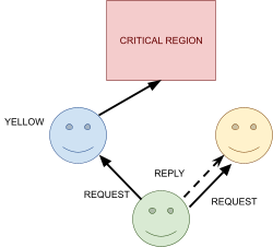
Leader Election
Assumptions:

N processes with unique, totally ordered IDs
Messages are eventually delivered (no failed packets)
Process with highest ID must win the election

Correctness:

Safety: a participant’s vote must either be or P (where P is non-crashed process with highest ID)
Liveness: all processes participate & eventually set their vote to something other than (or they crash)

Ring-based algorithm

Bully election algorithm

Pass ELECTION and ELECTED messages around in a ring, updating the process ID inside it. Used in asynchronous systems.

safety
liveness
does not tolerate failures (however we can modify to use a list, which mitigates this)
O(N) in both worst and best case

When a coordinator fails, failure detection systems fire off in other nodes and they send ELECTION and COORDINATOR messages to decide the new coordinator. Used in synchronous systems.

no safety
liveness
O(N2) worst case, O(N) best case

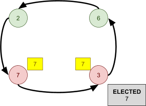
Reliable and Ordered Multicast
Closed group: only members can multicast
Open group: anyone can multicast

Basic multicast: sends messages directly to all participants. No specific order or reliability
Reliable multicast: basic multicasts, then everyone who receives a new message basic multicasts that too. Ensures reliability. It’s what we implemented in the second coursework.
Ordered multicast: a multicast that ensures some form of order

FIFO order: messages sent before other messages must come first. Process-specific sequence numbers are used.
Causal order: extension of FIFO, but uses causal relation (includes concepts like responses). Vector timestamps are used.
Total order: all messages received in the same order by all processes. Group-specific sequence numbers are used. Impossible to use in asynchronous system, because total order can solve consensus.

Consensus
Byzantine failures: processes lying/giving false information in a consensus algorithm
Solve consensus => can solve RTO multicast
Solve RTO multicast => can solve consensus

In synchronous systems, we can use 2PC to get consensus
Impossible to get consensus if , where N is processes and f is number of liars. Called Byzantine generals problem.

In asynchronous systems, no algorithm for consensus
Can have almost-perfect algorithm, like modified ring-based algorithm

Consistency models

CP	Strong consistency (Google BigTable) Messages have global timestamps Order of messages respect timestamp Expensive, and not always necessary
	Sequential consistency Shuffles read and write operations together, like multi-threading or if a switch selects operations each iteration
	Strong eventual consistency Good compromise (don’t need to know this one)
	Causal consistency Uses the causal relation and vector clocks Operations are only in order by the causal relation Better performance than sequential
AP	Eventual consistency (Amazon Dynamo) Lazy; eventually update replicas Can have conflicts, so we can use consensus or roll back

Leonardo’s stuff

Data Replication and Scalability
Primary-backup: one primary server, many back-up servers. Back-up servers are updated with updates passed to primary server.

Bottleneck: primary and back-up servers
Mitigation:

Share data on lots of primary servers, but we’ll need coordination.
Primary server only waits for some ACKs, but not all back-ups may be up-to-date.

CAP theorem: Pick two out of three:

Consistency
Availability
Partition tolerance

Assessing scalability:

Scale parameters: raw data that changes over time
Scalability metrics: measurements of parameters
Scalability criteria: conditions based on metrics that should be true

Highly Available Distributed Data Stores (Amazon Dynamo)
Amazon Dynamo: key-value store based on a ring architecture (distributed hash table).
Preference list: list of nodes responsible for a key. More than N
Request coordinator: first non-faulty node in the preference list

Three parameters:

N - number of nodes to request reads/writes
W - number of expected nodes to respond to writes
R - number of expected nodes to respond to reads

- can return stale versions of the object
- when we read, we can get multiple versions
- optimise reading
- optimise writing

How to diverge branches:

Syntactic reconciliation: if new version subsumes previous version, simply merge
Semantic reconciliation: send branches to client to decide. Uses vector clocks with node ID and update count pairs

Sloppy quorum: if node in preference list dies, pick a node outside N but within preference list to update and remind dead node when it comes back online (called hinted handoff)
Replica synchronisation: periodic protocol runs in background and ensures everything is synced. Based on Merkle trees.

Why AP: sloppy quorum lets Dynamo run even when nodes go down. There are conflicts, so it’s not CP

Bottleneck: all the nodes, collectively
Mitigation: add more nodes

Scalability: adding nodes is easy, the following nodes gives the new node the keys they’re not in charge of anymore

Consistent Distributed Data Stores (Google BigTable)
Google BigTable: table-based store that splits up columns into families

Rows of families => stored in tablets
Tablets => stored in tablet servers
Tablet servers => managed by master server
Tablets point to SSTables with data in chunkservers

GFS (Google File System): file system that BigTable uses
Files => divided into chunks
Chunks => replicated onto chunkservers
Chunkservers => managed by master server

Chubby: highly available config server storing files, directories, parameters, tidbits to help BigTable run

Tablet levels:

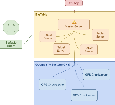
First level: Chubby -> root tablet
Second level: Root tablet -> METADATA tablets
Third level: METADATA tablets -> user data tablets

Master server and tablet servers have their own locks in Chubby

SSTable (Sorted Strings Table): file format used by BigTable to store data
Immutable ordered key-value
Split up into blocks

memtable is buffer, SSTable store locked immutable changes
writes: goes to memtable, reads: merge memtable and SSTables together to read

Minor compaction	Major compaction
Empty out memtable into new SSTable	Compress all SSTables and memtable into one big SSTable

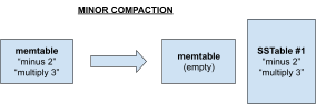
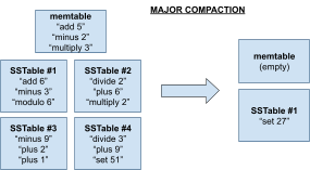
Why CP: if master dies, no requests, or when tablet server dies, tablet cannot serve requests; less availability
GFS is copy-on-write, so reads/writes are serialised, no race conditions, more consistency

Bottleneck: tablet servers and GFS chunkservers
Mitigation: add more tablet servers / chunkservers, but then master will become bottleneck

Online Distributed Processing
Apache Storm: used to handle streams of incoming data / events
Spout: outputs raw data
Bolt: modifies data in some way and passes it on / stores it

One master node, many worker nodes
Master node runs Nimbus process, which has a scheduler
Worker nodes have a supervisor with many executors (threads) running worker processes
Whole thing is called a cluster.

Replication: pipelining stateless operations to distribute workload
Grouping strategies:

Shuffle: random
Fields: based on fields predicate
All: all data is sent on all pipes
None: don’t care
Direct: producer picks explicitly
Local or shuffle: pipe data to nodes running on same worker node

Bottleneck: CPU / memory of overloaded spout/bolts.
Mitigation: increase replication factor or add more worker nodes

acker monitors DAG of input tuple and prunes DAG when bolt acks acker.
When DAG is empty, acker sends message to spout saying input processing was successful
When timeout, acker sends message to spout saying it’s failed. Spout may repeat input.

Batch Distributed Processing
We store data instead of processing it straight away
Not suitable for real-time systems
Uses splitting -> map -> shuffling -> reduce procedure

Google MapReduce: implementation of batch distributed processing

Apache Hadoop: another implementation of batch distributed processing
JobTracker -> delegates jobs to TaskTrackers
TaskTracker -> delegates tasks to task processes

Bottleneck: task tracker, if too many tasks
Mitigation: add more task trackers. If we add too many, job tracker will be bottleneck

HDFS (Hadoop Distributed File System): file system used by Hadoop, designed for single writer multiple reader
Data => divided into chunks
Chunks => replicated over DataNodes
NameNode => decides which chunk goes in which DataNode

Locality awareness: job tracker assigns mappers to task trackers with data nodes storing the data they need

Task fails: Job tracker detects it, moves it to another task tracker
Task tracker fails: blacklisted, all tasks moved to another task tracker
Job tracker fails: you’re stuffed; single point of failure

🎊 You’ve reached the end. Good luck on the exam! 🎊