Algorithmic Game Theory
Matthew Barnes
Normal / Extensive Form Games 3
Intro to Algorithmic Mechanism Design 7
Dominant-Strategy Truthfulness 18
Vickrey-Clarke Groves (VCG) Mechanism 19
Direct Quasilinear Mechanisms 19
Vickrey-Clarke-Groves (VCG) Mechanisms 22
Characterisation of DS Truthful Mechanisms 34
Dominant Strategy Implementation 36
The Case for Unrestricted Quasilinear Settings 38
The Case for Single Dimensional Settings 40
Example of an Optimal Auction 44
GS Returns Stable Matching Proof 52
Extensions of Stable Matching 53
Hospital Residents Problem (HR) 60
Hospital Residents Problem with Couples (HRC) 65
You Request My House - I Get Your Turn (YRMH-IGYT) 77
Probabilistic Serial Mechanism 82
Optimal k for smaller values of n 89
Arrow’s Impossibility Theorem 91


|
|
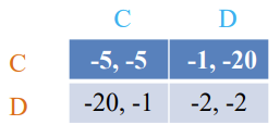
Payoff matrix for row player
|
|||||||||
|
Payoff matrix for column player
|
 : row player strategy, probability of playing pure strategy

 : column player strategy, probability of playing pure
strategy
: column player strategy, probability of playing pure
strategy


 is Nash equilibrium if:
 , then
 , then
 ⇒ pure strategy
 ⇒ mixed strategy
is a mixed Nash equilibrium if every pure strategy in  is a best response to
  and vice versa.
 where
where  ,
(possibly mixed) such that
,
(possibly mixed) such that
 is a Nash equilibrium.
|
Primal problem |
Dual problem |
|
max
s.t.
|
min
s.t
|
, 

 is the opt solution of Primal, and
  is the opt solution of Dual, then
is a Nash equilibrium of the game if:
, then  , then
  is an ε-Nash equilibrium of the game if:
, then
is an ε-Nash equilibrium of the game if:
, then 

 , then

 assigning each outcome a real number, so for any two
outcomes,
assigning each outcome a real number, so for any two
outcomes, 
|
Example 1994 Carribean cup qualification |
|
Bahar likes football, so football examples it is.
|
summary pls Auctions |
|

 is a finite set of agents
 is the set of all action profiles, where
  is the set of actions for agent .
 , where
  (reals) is the utility for agent .
 is a finite set of agents
, is the set of all action profiles, where is the set of actions for agent .
is a finite set of agents
, is the set of all action profiles, where is the set of actions for agent .
 is the set of all type profiles, where
  is the type space of player .
 is a common-prior probability distribution on
  .
, where
.
, where  (reals) is the utility for agent .
is the set of all possible types that player could have, so  .
’s type is chosen according to the
.
’s type is chosen according to the  probability distribution over .
|
|
💡 NOTE |
|
|
|
There are three stages of a Bayesian game:
Ex-ante: the player knows nothing about anyone’s types, even their own Interim: the player knows their own type, but nobody else’s. Ex-post: the player knows all players’ types.
Typically, when we reason with Bayesian games, we’re referring to the interim stage.
For more information, I suggest checking out this cheat sheet. |
|
. So they could make educated guesses.
is not known; that is, we have no probabilistic
information in the model.
|
Example Sheriff’s Dilemma Part 1: Phantom Bayesian Game |
||||||||||||||||||||||||||||
|
||||||||||||||||||||||||||||
pew pew 🔫
 where:
is a finite set of agents
where:
is a finite set of agents
 is a set of outcomes
where i is the type space of player i.
is a common-prior probability distribution on
, where
is a set of outcomes
where i is the type space of player i.
is a common-prior probability distribution on
, where 
 (reals) is the utility function for player .
) is a pair  where:
where is the set of actions available to agent
where:
where is the set of actions available to agent
 maps each action profile to an outcome
 , which returns a probability distribution over the
outcomes. However, we’ll focus on just deterministic
mechanisms for now.
, which returns a probability distribution over the
outcomes. However, we’ll focus on just deterministic
mechanisms for now.
The only action available to these gears
in this mechanism is to keep on turning.
 for each .
where:
where is the set of actions available to agent
maps each action profile to an outcome
for each .
where:
where is the set of actions available to agent
maps each action profile to an outcome
 (realsn) for a finite set of choices


 is chosen, the utility of an agent given type
  is
is 

 , is the result of the optimisation problem of our
mechanism.
, is the cost of this outcome for each player .
, is the result of the optimisation problem of our
mechanism.
, is the cost of this outcome for each player .
’s utility function as  .
for choice as
.
for choice as  .
of an outcome
.
of an outcome  is their valuation minus their payment:

|
|
💡 NOTE |
|
|
|
Remember that the type isn’t always just the valuation!
The valuation
The type
The valuation isn’t the type, but the valuation does depend on the type. |
|
 is where
is the set of action profiles where is the set of actions available to player .
is where
is the set of action profiles where is the set of actions available to player .
 is the choice function that maps action profiles to choices.
 (realsn) is the payment function that maps action profiles to payments for each
agent.
(realsn) is the payment function that maps action profiles to payments for each
agent.
|
Example Sheriff’s Dilemma Part 2: Bayesian Game Setting and Mechanism Tendency |
|
(where  )
)


 where:
 is a utility function defined as


Bayesian Game Setting + Mechanism = Bayesian Game
 such that each
  is a best response to
  .
over the types .
.
over the types .
|
summary pls Social Choice setting |
|
 vanilla chocolate) and the result is based purely off of those
preferences.
vanilla chocolate) and the result is based purely off of those
preferences.
strictly dominates  if for all
  it is the case that
  weakly dominates if for all it is the case that
  , and for at least one it is the case that
very weakly dominates if for all it is the case that
, and for at least one it is the case that
very weakly dominates if for all it is the case that
|
|
💡 NOTE |
|
|
|
For all the above cases, we say that strictly dominated strategy if another strategy strictly dominates it.
A strategy is strictly dominant for an agent if it strictly dominates all other strategies for that agent.
This is the same for weakly and very weakly dominance. |
|
implements a social choice function  in dominant strategies if for some dominant strategy equilibrium of the
induced game, we have that the mechanism chooses the same outcome (given action profile of the agents) as does (given true utilities of the agents).
in dominant strategies if for some dominant strategy equilibrium of the
induced game, we have that the mechanism chooses the same outcome (given action profile of the agents) as does (given true utilities of the agents).
 in which every is a dominant strategy for agent is called an equilibrium in dominant strategies.
, telling the truth (i.e. revealing the true valuation) maximises ’s utility, no matter what strategy the other players
pick.
is dominant-strategy truthful, then truth-telling (the action that correlates to your actual type) is always at least a very weakly dominant
strategy.
 .
, bidding
.
, bidding  maximises ’s utility, no matter what bids the other bidders
place:
maximises ’s utility, no matter what bids the other bidders
place:

will always be greater than the utility of any bid
other than , no matter what bids our opponents make.
will always be greater than the utility of any bid
other than , even if all the opponents play truthfully.
If you’re playing a Bayesian game with a dominant-strategy
truthful mechanism, you should tell the truth.
 where:
 is the choice function that maps type spaces to choices.
 (realsn) is the payment function that maps type spaces to payments for each
agent.
(realsn) is the payment function that maps type spaces to payments for each
agent.
 , we can substitute the two in a quasilinear mechanism to
get a direct quasilinear mechanism.
.
, we can substitute the two in a quasilinear mechanism to
get a direct quasilinear mechanism.
.
 .
.
 for every choice
  .
.
 , whereas our actual, true valuations are labelled
  .
.
 .
.
 denotes the declared valuations of everyone except
agent .
denotes the declared valuations of everyone except
agent .
|
Property |
Definition |
English pls |
|
(Strict Pareto) Efficiency Social-welfare maximising |
A quasilinear mechanism is efficient (or social-welfare maximising) if, in equilibrium, it selects a choice |
It picks the choice that maximises the sum of everyone’s valuations for that choice. |
|
Dominant-strategy truthful Tell the truth |
A direct quasilinear mechanism is dominant-strategy truthful (or just truthful) if for each agent |
Agents should declare their true valuation to maximise their utility. |
|
Ex interim individual rationality I won’t lose |
A mechanism is ex interim individually rational if, in equilibrium, each agent
Formally, it’s when
where |
No agent will receive negative utility, calculated using an average estimate of everyone else’s valuations.
This is weaker than ex post individual rationality, so: Ex-post IR ⇒ Ex-interim IR.
Why do we estimate? The “interim” stage means the player knows their own type (valuation), but not anybody else’s. Therefore, to calculate their utility in this stage, they must estimate everyone else’s valuations using a known distribution. |
|
Ex post individual rationality No-one will lose |
A mechanism is ex post individually rational if, in equilibrium, the utility of each agent is at least 0.
Formally, it’s when
where |
No agent will receive negative utility and lose by participating in the mechanism.
In the “ex-post” stage, everyone knows everybody’s valuations. Therefore, true utilities can be calculated without estimations. |
|
Budget balance Mechanism breaks even |
A quasilinear mechanism is budget balanced when |
The mechanism won’t receive any profits or losses; it’ll break even. |
|
Weakly budget balance Mechanism breaks even or profits |
A quasilinear mechanism is weakly budget balanced when |
The mechanism won’t lose money; it’ll only profit or break even. |
|
Tractability Feasible to run |
A quasilinear mechanism is tractable if for all |
It’s computationally feasible; the algorithm complexities are fast enough to run and be used in-practice. |
defined as follows:


 uses
uses  to select the choice that maximises the sum of all declared valuations for
that choice (a.k.a, the social-welfare), making Groves mechanisms efficient.
to select the choice that maximises the sum of all declared valuations for
that choice (a.k.a, the social-welfare), making Groves mechanisms efficient.
 agent :
 term)
must pay that doesn’t depend on their own
valuation.
term)
must pay that doesn’t depend on their own
valuation.
|
Theorem Green-Laffont |
|
In settings where agents may have unrestricted quasilinear utilities, Groves mechanisms are the only mechanisms that are both:
Here’s the formal statement if you want:
Suppose that for all agents any |
where:

 .
.
|
|
💡 NOTE |
|
|
|
VCG is a specific mechanism within the class of Groves mechanisms (the most famous mechanism within this class).
Some people refer to Groves mechanisms as VCG mechanisms (which is confusing IMO).
Vickrey auction is a special case of VCG, and hence VCG is sometimes known as the “generalised Vickrey auction”.
In fact, single-item VCGs are literally just Vickrey auctions! |
|
|
|
Optimal social welfare of other agents
if agent |
|
Optimal social welfare of other agents
if agent |
is greater than 0:
.
is 0:
is less than 0:
.
|
|
|
|
|
|
Remember from quasilinear utility settings? Utility is:
If we substitute everything with VCG stuff, we can represent utility in terms of social welfare.
Outcome
Choice
Type
The utility is the social welfare of the
current choice minus the social welfare if agent |
|
|
Example VCG In Action: Auction |
||||||||||||
|
|
Example VCG In Action: Vickrey Auction |
|||||
|
|
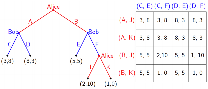
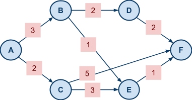
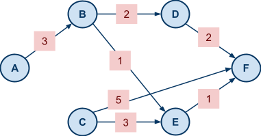
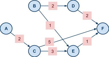
Example VCG In Action: Shortest Path |
|
 picks some arbitrary strategy
  (they don’t have to be truthful).
is still deciding in their strategy .
is one that solves:
(they don’t have to be truthful).
is still deciding in their strategy .
is one that solves:

that maximises agent ’s utility.

 has nothing to do with , so it’s virtually a constant in this setting.
It’s sufficient just to solve:
has nothing to do with , so it’s virtually a constant in this setting.
It’s sufficient just to solve:

influences this maximisation is through the choice the mechanism picks. So would like to pick a strategy that will lead the mechanism to pick a choice that solves:


 .
.
.
.
|
|
💡 NOTE |
|
|
|
VCGs may seem like the best thing ever, right?
Well, it’s rarely used in practice.
This is because it has a long list of weaknesses.
One of its biggest weaknesses is that finding the social-welfare maximising choice might be NP-hard, so it doesn’t have tractability (not feasible). This is especially true in combinatorial auctions. |
|
|
Property |
Definition |
English pls |
|
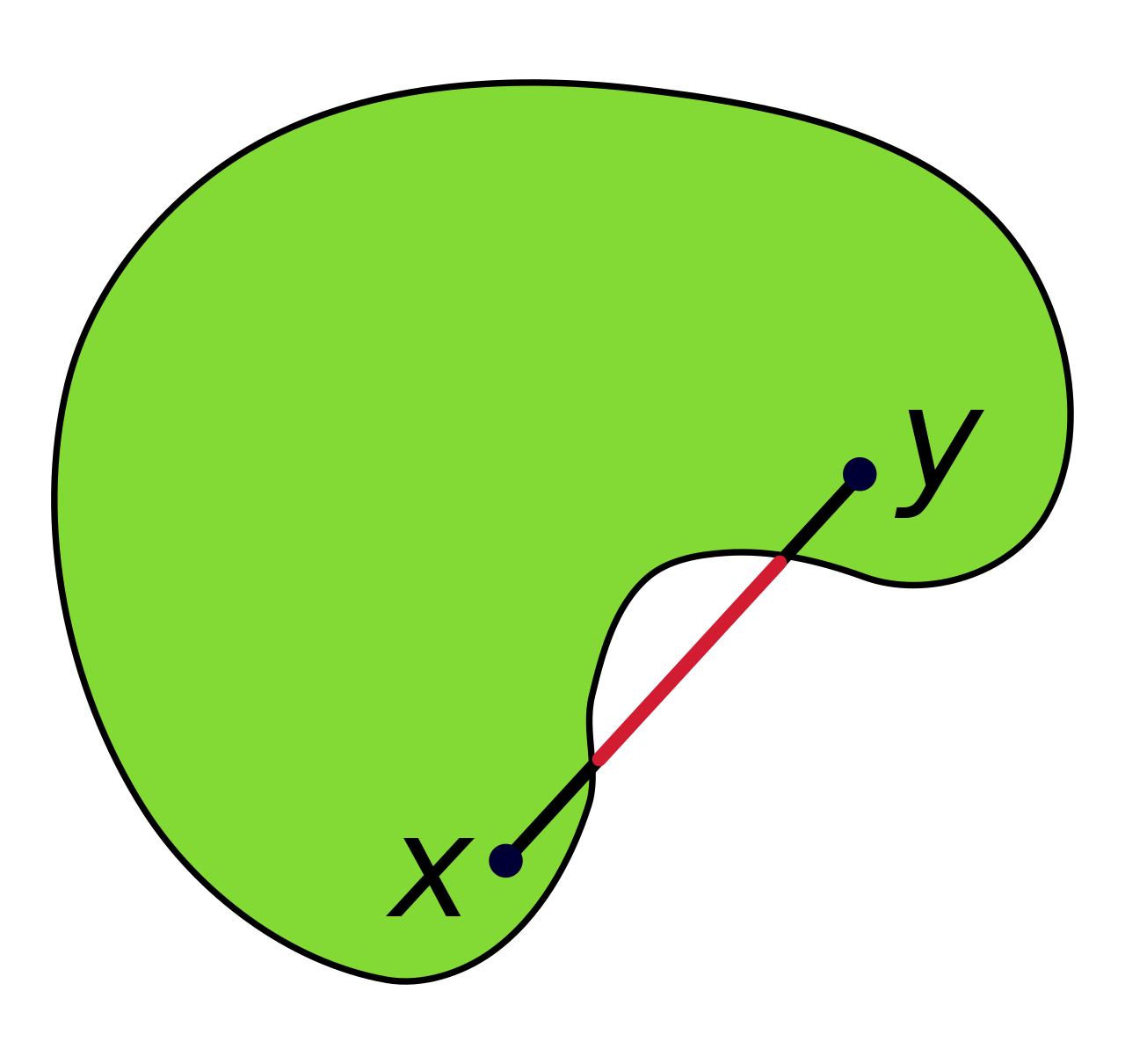
Choice-set monotonicity Less people, same/less choices |
A setting exhibits choice-set monotonicity if |
Removing an agent will never grant more choices. |
|
No negative externalities No participation? No worries! |
A setting exhibits no negative externalities if |
Every agent has zero or positive utility for choices made without their participation. |
|
Theorem |
|
The VCG mechanism is ex-post individual rational when the choice-set monotonicity and no negative externalities properties hold. |
 in terms of social welfare” note above, our
utility can be expressed as:
in terms of social welfare” note above, our
utility can be expressed as:

 maximises social welfare, meaning its social welfare
is at least as big as
maximises social welfare, meaning its social welfare
is at least as big as  ’s social welfare. Because of choice-set
monotonicity, no better choice would appear without agent . We can represent that as:
’s social welfare. Because of choice-set
monotonicity, no better choice would appear without agent . We can represent that as:

has zero / positive utility on a choice made without
their participation. We can represent that as:


 is positive, we can subtract it from the right side
and the equality will still hold:
is positive, we can subtract it from the right side
and the equality will still hold:

|
Property |
Definition |
English pls |
|
No single-agent effect Please leave. |
A setting exhibits no single-agent effect if |
Welfare of agents other than
Example: In an auction setting, agents are better off when one other agent drops out, because there’s less competition.
Therefore, auction settings exhibit no single-agent effect. |
|
Theorem |
|
The VCG mechanism is weakly budget-balanced when the no single-agent effect property holds. |


should be greater than the social welfare of the
choice with , because everyone is better off removing other
agents:

|
Theorem Krishna & Perry, 1998 |
|
In any Bayesian game setting in which VCG is ex post individually rational...
... VCG collects at least as much revenue as any other efficient and ex interim individually-rational mechanism. |
|
Theorem Green-Laffont; Hurwics |
|
No dominant-strategy truthful mechanism is always both efficient and weakly budget balanced, even if agents are restricted to the simple exchange setting. |
|
Theorem Myerson-Satterthwaite |
|
No Bayes-Nash incentive-compatible mechanism is always simultaneously efficient, weakly budget balanced and ex interim individually rational, even if agents are restricted to quasilinear utility functions. |
“People die if they are killed”
|
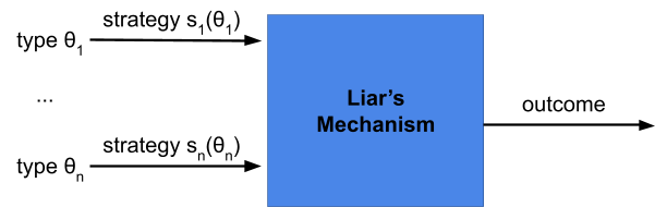
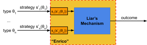
Theorem Revelation Principle |
|
For every mechanism in which every participant has a dominant strategy (no matter what their private information), there is an equivalent direct dominant-strategy truthful mechanism. |
has a strategy function that, given a type, plays a dominant
strategy (not a truthful one).
.
 denote the set of choices that can be selected by the
choice rule
denote the set of choices that can be selected by the
choice rule  given the declaration by the agents other than (i.e. the range of
  ).
).
|
Theorem |
|
A mechanism is dominant-strategy truthful if
and only if it satisfies the following
conditions for every agent
1. The payment function
2.
|
has already decided and locked in their
strategy.
 is the set of choices that the mechanism may pick,
depending on agent ’s final decision.
still indirectly affects the payment, but only
through the choice of the mechanism.
’s point of view, the mechanism always selects the
choice that maximises their utility (in other words, the mechanism optimises for each
agent).
is the set of choices that the mechanism may pick,
depending on agent ’s final decision.
still indirectly affects the payment, but only
through the choice of the mechanism.
’s point of view, the mechanism always selects the
choice that maximises their utility (in other words, the mechanism optimises for each
agent).
|
If part |
Only if part |
||||||||
|
Let’s say that agent
Now, let’s walk through what’s
going to happen to agent
If
If
If
Therefore, it’s a dominant strategy for |
First condition:
Let’s assume, for the sake of
contradiction, the payment function did depend
on
That means there could be a truthful strategy
Then
So, as per this proof by contradiction, the
payment cannot depend on
Second condition:
Again, for the sake of contradiction,
let’s say player
That means there could be some other untruthful
valuation
Then
As per this proof by contradiction, the mechanism must pick the choice that maximises utility if this mechanism is DS truthful. |
|
Property |
Definition |
English pls |
|
Weak Monotonicity WMON |
A social choice function |
Let’s say the mechanism picks
When an agent |
|
Theorem WMON is necessary for DS truthfulness |
|
If a mechanism
DS truthful → WMON |
|
Theorem When WMON is sufficient for DS truthfulness |
|
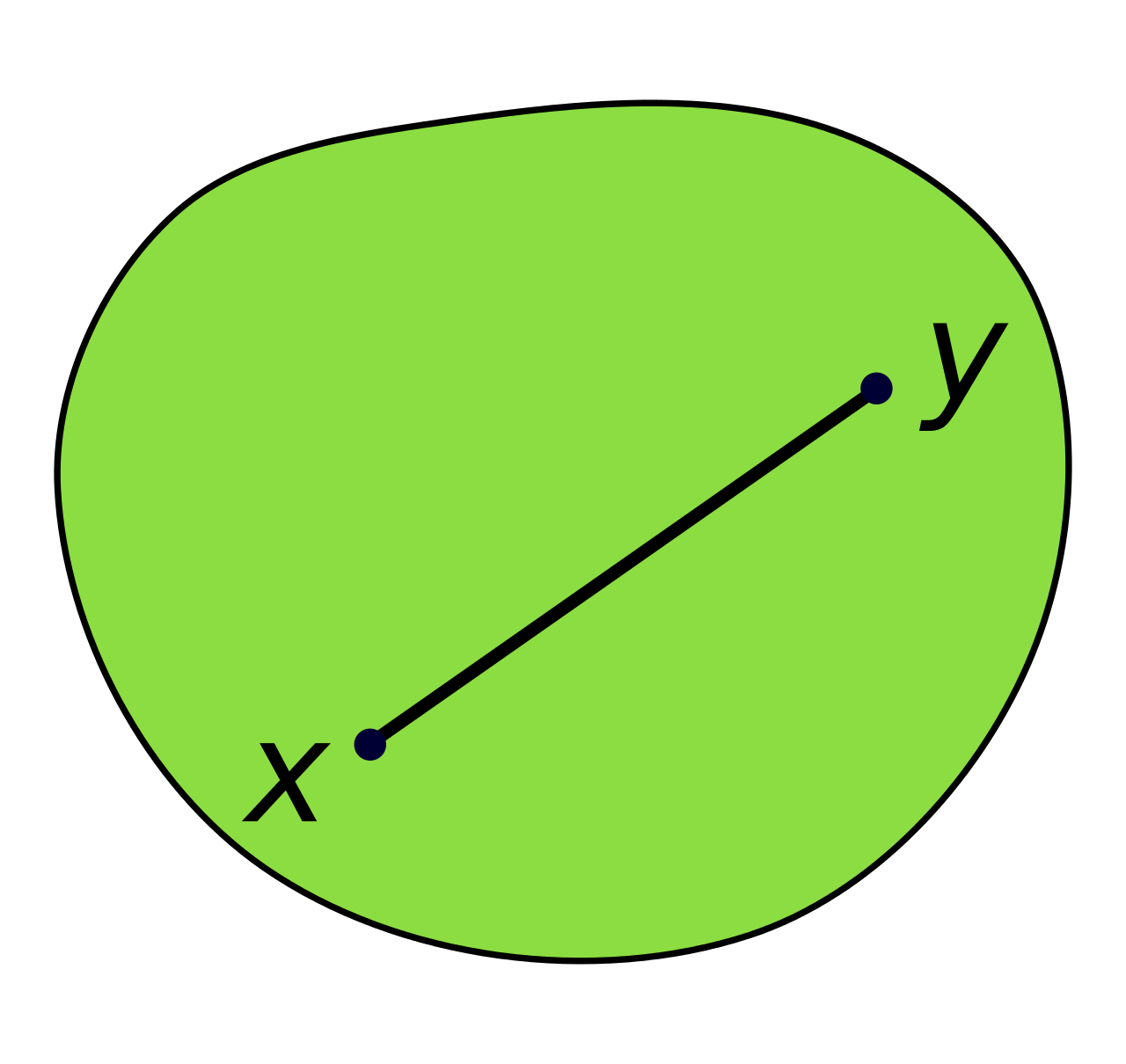
If all domains of preferences
WMON → DS truthful (if preferences are convex sets) |
 are convex sets, then every WMON social choice has
payment functions such that the mechanism is DS
truthful.
are convex sets, then every WMON social choice has
payment functions such that the mechanism is DS
truthful.
|
Wahoo yes convex set 🎉🎉🎉🎉 |
Boo no convex set 😡💢💢 |
|
|
|
 (set of reals)
is an affine maximiser if for some subrange
(set of reals)
is an affine maximiser if for some subrange  , for some agent weights
  (set of positive reals), and for some outcome weights
  ,
, , has the form:

 have weights,
  .
.
 .
.
 .
.

|
|
Affine maximisers = DS truthful? |
|
|
|
“Any affine maximiser social choice
function
Can we prove it? You bet we can!
VCG is truthful. What if we just stick the affine maximiser choice function into VCG and see if that works?
On the right track, but... hmm, no. That doesn’t feel right. It’s not rigorous enough.
Let’s have a closer look at what makes VCG and affine maximisers different.
Let’s take the choice function of VCG and abstract it a little:
Here, I’ve defined a social welfare
Now, how do we “transform” our VCG to an affine maximiser?
We should create a new, refined
Can you see how substituting our new
Well, we’ve substituted it in the choice
function. The payment function used
There we have it! A payment function that, when
paired with its respective affine maximiser
We could factor out
(what, you thought I came up with this on my own?) |
|
|
Theorem Roberts |
|
If there are at least three choices that a social choice function will choose given some input, and if agents have general quasilinear preferences, then the set of (deterministic) social choice functions implementable in dominant strategies is precisely the set of affine maximisers. |
), the only DS-implementable social choice functions are
affine maximisers.
 and
and  .
.
.
 (where
  ) that are all equivalent to each other in terms of
value to agent . Choices
) that are all equivalent to each other in terms of
value to agent . Choices  yield a value of 0.
wins.
yield a value of 0.
wins.
 is a singleton, with the choice where wins the item.
contains choices where the agent gets their bundle
and/or more.
is a singleton, with the choice where wins the item.
contains choices where the agent gets their bundle
and/or more.
has winning alternatives and a range of values  , which are both publicly known.
 and
and  are used as lower and upper bounds for the valuation , but don’t worry; they’re not important
here.
values all at (which is private knowledge), and 0 for everything else.
are used as lower and upper bounds for the valuation , but don’t worry; they’re not important
here.
values all at (which is private knowledge), and 0 for everything else.
|
Property |
Definition |
English pls |
|
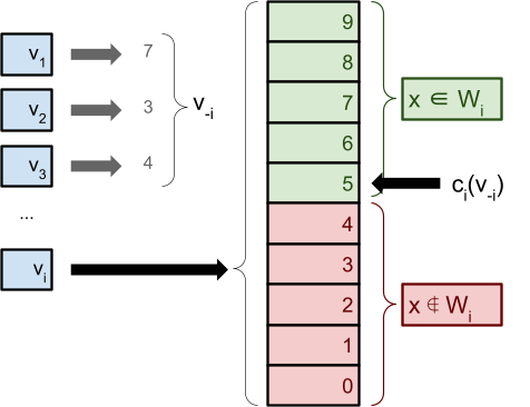
Monotonicity
Monotone in |
A social choice function |
If agent |
, for every  for which agent can both win and lose, there is always a critical
value
for which agent can both win and lose, there is always a critical
value  below which loses and above which they win.
wins for every , then the critical value at is undefined.
 if
if  .
.
|
Theorem |
|
A normalised mechanism
|


Economists designing optimal auctions
’s valuation is drawn from some strictly increasing
cumulative density function  with a PDF (probability distribution function)
  that is continuous and bounded below.
 (asymmetric auctions)
 .
is uniformly distributed on
.
is uniformly distributed on  (each possible valuation has an equal chance of being
picked).
(each possible valuation has an equal chance of being
picked).
 between 0 and 1, where:
if there’s one bid below and one above
will maximise expected revenue?
makes this an optimal auction? 🤔
between 0 and 1, where:
if there’s one bid below and one above
will maximise expected revenue?
makes this an optimal auction? 🤔
Buy BaharCoin while it’s still low
|
1. Both bids are below |
|
The chance of one valuation being drawn below
Probability:
Revenue: |
|
2. One bid is below |
|
The chance that one valuation is drawn above
The first case is player 1’s valuation
being drawn below
The second case is the opposite: player
2’s valuation being below and player
1’s being above. The probability of that
is also
Either the first case could happen OR the
second case, so we add them up (both cases are mutually exclusive) to get the total probability that one bid
is below and one is above:
Probability:
Revenue: |
|
3. Both bids are above |
|
Both players draw valuations above
The expected revenue of this case is derived
from the expected minimum valuation drawn, given
that both bids are above
If you want to know why it’s
Probability:
Revenue: |


 (Careful! There’s two turning points; this is the
maximum, but the other (
(Careful! There’s two turning points; this is the
maximum, but the other ( ) is a minimum.)
.
) is a minimum.)
.
 , the seller will get on average
  BaharCoin.
 , the seller will get on average
  BaharCoin.
, but it would’ve been low revenue anyway and
that’ll only happen
BaharCoin.
, but it would’ve been low revenue anyway and
that’ll only happen  of the time.
of the time.
of the time.
’s virtual valuation is  .
(every time goes up, the virtual valuation
.
(every time goes up, the virtual valuation  will go up too)
 .
.
.
.
’s bidder-specific reserve price  is the value for which
  .
.
|
Theorem Myerson (1981) |
|
The optimal (single-item) auction is a sealed-bid auction in which every agent is asked to declare their valuation.
The good is sold to the agent
If the good is sold, the winning agent
|
|
|
You heard it here first, folks: Google’s optimal sock auctions.


 wants to deviate
|
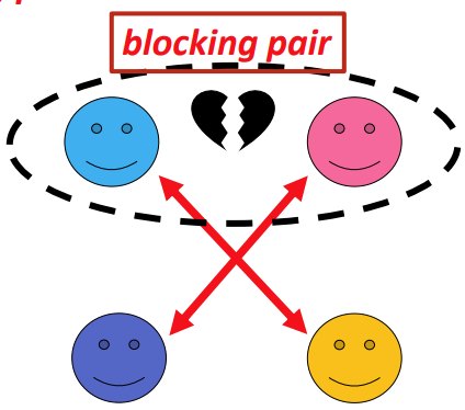
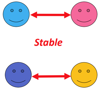
Let’s say there’s two leaders, red and orange, and two followers, blue and purple.
They have the following preferences:
In summary, red is the most popular leader, and blue is the most popular follower.
It makes sense that the most popular leader and follower would want each other.
However, check out the pairing on the right: blue is paired with orange, and red is paired with purple.
Blue and red would rather be paired with each other. This is a blocking pair. |
|
||||
|
|
Now, look at the pairing on the left. Blue and red are now paired, so it’s not a blocking pair anymore.
Sure, purple would rather be with red, and orange would rather be with blue, but blue and red are happy where they are, so those aren’t blocking pairs. |
|
Theorem Myerson (1981) |
|
A stable matching always exists, and can be found in polynomial time. |
|
Gale-Shapley algorithm pseudocode (leader-oriented) |
|
Assign all leaders and followers to be free // Initial state
|


 a blocking pair?
 prefer
  to its current matching,
  ?
’s preferences, is before .
prefers .
prefer to its current matching,
?
’s preferences, is before .
prefers .
prefer to its current matching,  ?
’s preferences, is before .
prefers .
is a blocking pair.
?
’s preferences, is before .
prefers .
is a blocking pair.
a blocking pair?
prefer to its current matching, ?
prefer to its current matching, ?
|
1. The algorithm always terminates |
2. The algorithm returns a matching |
3. The matching it returns is stable |
|
We notice two things about GS:
Because of this, the algorithm terminates after
at most
Why?
Because for each leader, they propose to
This is also a proof for GS being in polynomial time. |
In this proof, we’ll show that GS returns a one-to-one matching, meaning that each leader has at least one follower and vice versa.
This will be split into two parts:
1. In GS, all leaders get matched. Let’s do a proof by contradiction.
Let’s say there’s some leader
That means there must be some follower
If
But, A contradiction!
2. In GS, all followers get matched. As proved before, all leaders get matched.
If all
But Therefore all followers must be matched. |
We can prove that the returned matching
Consider any pair
There are two possibilities for the pair
1.
2.
In either case, |
|
Gale-Shapley algorithm pseudocode (leader-oriented, SMI) |
|
Assign all leaders and followers to be free // Initial state
|
No! 🤦♂️ It’s not where we match office ties...
:
 strictly prefers to their current follower, and strictly prefers to their current leader
strictly prefers to their current follower, and is indifferent between and their current leader
is indifferent between and their current follower, and strictly prefers to their current leader
strictly prefers to their current follower, and strictly prefers to their current leader
strictly prefers to their current follower, and is indifferent between and their current leader
is indifferent between and their current follower, and strictly prefers to their current leader
and are achievable to .
is achievable to  .
and a follower are achievable if there exists some stable matching where and are matched.
.
and a follower are achievable if there exists some stable matching where and are matched.
|
Proof |
|
So our claim was “leader-oriented GS’ return leader-optimal matchings”.
To do a proof by contradiction, we need to consider “a leader-oriented GS does not return a leader-optimal matching”.
Leaders propose in decreasing order of preferences, so therefore some leader is going to be rejected by an achievable partner during GS (this doesn’t always happen, but it happens most of the time. We’ll consider it in this example).
Let’s say we have some leaders and some followers, and we’re running a GS.
All of the sudden, some leader
Since
Now, when
We now know
In our ‘other’ stable matching,
When
So,
If
Why? Because if they preferred
We now know
Let’s summarise what we’ve found out so far:
There is a blocking pair:
Therefore, leader-oriented GS’ must return leader-optimal matchings. |
|
When preferences are strict, all executions of leader-oriented GS return the same stable matching. |
When preferences are strict, there exists:
|
|
Theorem Myerson (1981) |
|
When preferences are strict, the leader-optimal matching is the follower-pessimal matching, and vice versa. |
 prefers purple, but prefers green
prefers green, but prefers purple
prefers purple, but prefers green
prefers green, but prefers purple
|
Theorem Dubins and Freedleader; Roth |
|
The mechanism that yields the leader-optimal stable matching (in terms of stated preferences) makes it a dominant strategy for each leader to state their true preferences. |
|
Theorem Roth, 1982 |
|
No stable matching mechanism exists for which truth-telling is a dominant strategy for every agent. |
|
Theorem Roth and Sotomayor, 1990 |
|
When any stable mechanism is applied to a marriage market in which preferences are strict and there is more than one stable matching, then at least one agent can profitably misrepresent their preferences, assuming others tell the truth. |
|
Proof |
|
Here, we have two leaders and two followers:
This instance has two stable matching:
Every stable matching mechanism must choose either green or purple.
Suppose that our mechanism picks green.
Now, if
Similarly, if
In this scenario, at least one agent benefits by lying. |
|
Theorem Immorlica and Mahdian, SODA 2005 |
|
The number of students that have more than one achievable hospital vanishes. Therefore, with high probability, the truthful strategy is a dominant strategy. |
 students applying to universities.
 students.
, and not .
gets larger and larger, the proportion of such
students gets smaller and smaller, until it’s
practically zero.
students.
, and not .
gets larger and larger, the proportion of such
students gets smaller and smaller, until it’s
practically zero.
|
Theorem Gonczarowski and Friedgut, 2013 |
|
In an instance of SM (no ties or indifference), and assuming that lying is only possible by permuting one’s preferences: if no lying follower is worse off then
|
|
Problem |
Description |
|
SMI Stable Matching problem with Incomplete lists |
Agents may declare some candidates unacceptable, represented by preference lists of only some choices |
|
SMT Stable Matching problem with Ties Shin Megami Tensei |
Agents may be indifferent among several candidates |
|
SMTI Stable Matching problem with Ties and Incomplete lists |
Both incomplete lists and indifferences are allowed |
|
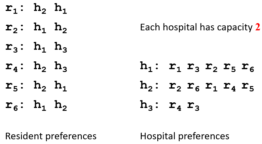
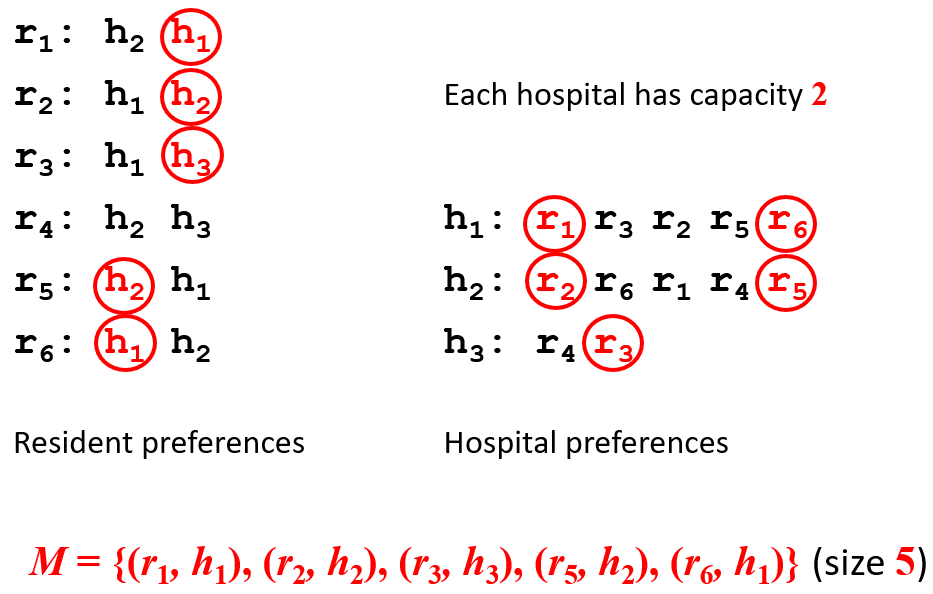
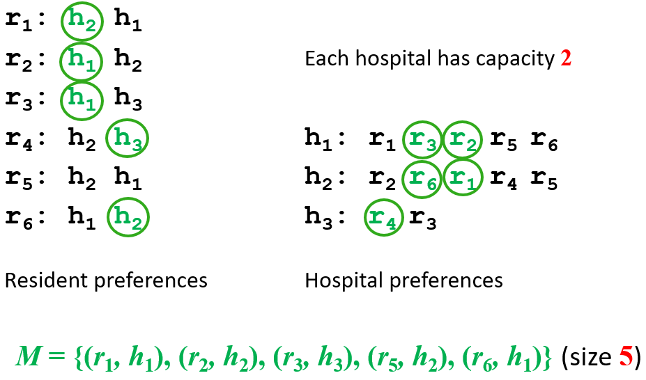
HR Hospitals / Residents problem |
Many-to-one stable matching problem with incomplete lists |
|
HRT Hospitals / Residents problem with Ties |
Many-to-one stable matching problem with ties and incomplete lists |
The namesake comes from junior doctors applying
and doing training in hospitals..
residents: 
 hospitals:
 and
and  find each other acceptable if they are in each others’ preference
lists.
finds unacceptable, then finds unacceptable.
find each other acceptable if they are in each others’ preference
lists.
finds unacceptable, then finds unacceptable.
is a set of resident-hospital pairs such that:
 find each other acceptable
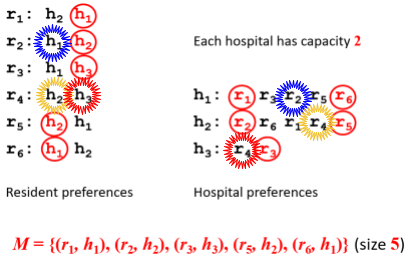
 is a blocking pair if:
and find each other acceptable
is unmatched in or
prefers to their assigned hospital in
is undersubscribed in or
prefers to its worst resident assigned in
is a blocking pair if:
and find each other acceptable
is unmatched in or
prefers to their assigned hospital in
is undersubscribed in or
prefers to its worst resident assigned in
 is a blocking pair because
  prefers
  to
to  , and prefers to
  .
.
 is a blocking pair because
  is unmatched, and prefers to
  .
.
 is a blocking pair because is unmatched, and
  is unmatched.
|
Resident-oriented Gale-Shapley algorithm pseudocode |
|
M = ∅ // assign all residents and hospitals to be free
while (some resident ri is unmatched and has a non-empty list) ri applies to the first hospital hj on their list M = M ∪ {(ri,hj)}
if (hj is over-subscribed) rk = worst resident assigned to hj M = M \ {(rk,hj)} // rk is set free if (hj is full) rk = worst resident assigned to hj for (each successor rl of rk on hj’s list) delete rl from hj’s list delete hj from rl’s list
output the engaged pairs, who form a stable matching |
|
Hospital-oriented Gale-Shapley algorithm pseudocode |
|
M = ∅ // assign all residents and hospitals to be free
while (some hospital hi is under-subscribed and has non-empty list) si = qi - |M(hi)| // the number of available seats in hi hi applies to the first si residents on its list
foreach (rj that hi applies to) if (rj is free) M = M ∪ {(rj,hi)} else if (rj prefers hi to her current hospital h’) M = M ∪ {(rj,hi)} \ {(rj,h’)} // h’ is set free if (rj is not free) for (each successor hl of M(rj) on rj’s list) delete hl from rj’s list delete rj from hl’s list output the engaged pairs, who form a stable matching |
Resident-optimal matchings and hospital-optimal matchings
|
Theorem Rural Hospitals Theorem (Roth, 1984; Gale and Sotomayor, 1985; Roth, 1986) |
|
In a given instance of HR:
|
 and the rest do not get assigned, then for all stable matchings in that HR problem, all residents in
  will be assigned and all other residents
  will not be assigned.
is the same.
who has matchings with
will not be assigned.
is the same.
who has matchings with  and is undersubscribed, then all stable matchings have the exact same matchings with for .
|
Theorem (Roth; 5.16 in TSM) |
|
A stable matching mechanism that yields the resident-optimal matching makes it a dominant strategy for all residents to state their true preferences. |
|
Theorem (Roth; 5.14 in TSM) |
|
No stable matching mechanism exists that makes it a dominant strategy for all hospitals to state their true preferences. |
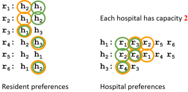
is stable in an HRT instance  if and only if is stable in some instance
  of HR obtained from by breaking the ties [Manlove et al, 1999].
 , that rank pairs of hospitals
  representing the assignment of
  to
to  and
and  to
to  .
.
|
(r1,r2): (h1,h2) r3 : h1 h2
h1: r1 r3 r2 h2: r1 r3 r2
Blocking pair: (r1,h1) |
(r1,r2): (h1,h2) r3 : h1 h2
h1: r1 r3 r2 h2: r1 r3 r2
Blocking pair: (r3,h1) |
(r1,r2): (h1,h2) r3 : h1 h2
h1: r1 r3 r2 h2: r1 r3 r2
Blocking pair: (r3,h2) |
|
[Ng and Hirschberg, 1988; Ronn, 1990] |
|
[Manlove and McBride, 2013] |
“What does that mean”, you may ask. I don’t know. I just write the notes. |
[Biró et al, 2011] [Manlove and McBride, 2013] |
 agents (or students)
 agents
is stable if there is no
agents
is stable if there is no  such that prefers
  to their current partner and vice versa.
 and
and  .
.
 !
!
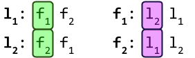
|
|
||
|
Let’s get all the matchings and show that none of them are stable. |
||
|
|
|
|
|
Blocking pair:
|
Blocking pair:
|
Blocking pair:
|
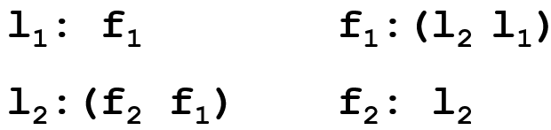
 , and works in two phases:
is engaged to , then that should mean is engaged to .
is engaged to , is not necessarily engaged to .
is semi-engaged to .
could either be:

(making them fully engaged)
A stock image of semi-engaged roommates.
|
Irving’s Algorithm Phase 1 pseudocode |
|
Assign all agents to be free // initial state
while (some free agent x has a non-empty list) y = first agent on x’s list
// next: x proposes y if (some person z is semi-engaged to y) assign z to be free // y rejects z
assign x to be semi-engaged to y
for (each successor w of x on y’s list) delete w from y’s list delete y from w’s list |
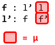
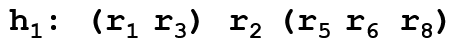
 where:
 is the second entry on ’s list, and
 is the last entry on ’s list
from ’s list
from ’s list
is the last entry on ’s list
from ’s list
from ’s list
|
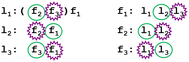
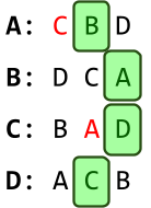
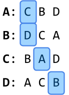
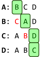
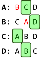
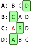
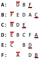
Intuitively, how do you find a rotation in a phase-1 table? |
|||||||
|
|
Alright, here’s a phase-1 table, and I’ll walk through how to find a rotation in it.
Let’s start at the top, with A, because A has a second preference:
A’s second preference is B, so we add B to the ‘q’ list:
Now, we look at B. B’s last preference is C, so we add C to the ‘p’ list:
We move on to C. C’s second preference is D, so we add D to the ‘q’ list:
Onto D. D’s last preference is A, so we add A to the ‘p’ list:
We’ve already got an A in the ‘p’ list! So, we stop there, or else we’d be repeating ourselves.
So, you see? We just alternate between putting the second preference in ‘q’ and the last preference in ‘p’ until we hit a cycle.
If we wanted to eliminate this rotation, we’d eliminate the bottom-left top-right pairs in these two sequences:
So, we’d remove |
||||||
|
Irving’s Algorithm Phase 2 pseudocode |
|
T = phase-1 table // initial state
while ((some list in T has more than one entry) and (no list in T is empty))
find a rotation
T = T /
if (some list in T is empty) return instance unsolvable else return T, which is a stable matching |
|
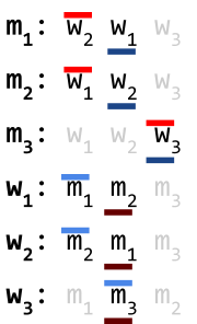
Starting our rotation with m1 |
Starting our rotation with w1 |
||||
|
Eliminated:
|
|
Eliminated:
|
|
||
Möbius strip matching: an alternative title.
agents, and houses.
Would you take part in a mechanism to
swap your house with someone else?
|
|
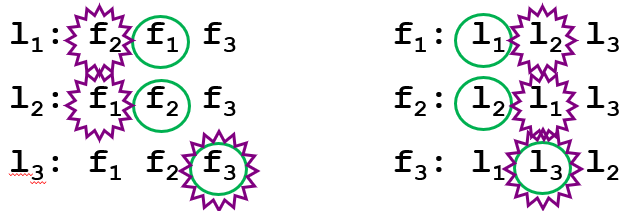
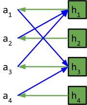
Here’s the preference lists:
a1 : h3 > h2 > h1 a2 : h1 > h4 > h2 a3 : h1 > h4 > h3 a4 : h3 > h4
The blue represents ownership, for example a1 owns h1.
On the diagram, the green arrows are the houses pointing to their owners, and the blue arrows are the agents pointing to their desired houses. |
|
|
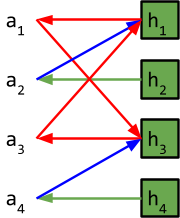
Now, we search for cycles. We start from one agent, and we follow through the arrows until we get back to the start.
Starting at a1, the following cycle can be found:
a1 → h3 → a3 → h1 → a1
So, we make the following assignment:
We remove these agents and houses from the algorithm, and we continue. |
|
|
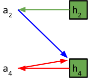
The houses a2 and a4 were pointing to are now allocated! So now, they point to the next available houses on their list.
Now, let’s look for another cycle:
a2 → h4 → a4 → h4
The cycle only loops around a4 and h4, so we’ll only assign a4 the house:
Now, we remove a4 and h4. |
|
|
It’s trivial that the only assignment left is to assign a2 to their own house!
So our final assignment is:
|
.
 , will they get a better house? No! They either get the
same one they would’ve got in round , or a worse one because their old house would have already
been taken.
, will they get a better house? No! They either get the
same one they would’ve got in round , or a worse one because their old house would have already
been taken.
students that have rooms,  .
newcomers
.
newcomers  .
vacant rooms
.
vacant rooms  .
.
 where
where  points to the house of agent
  , who points to the house of
  , and so on. In this case, assign these houses by letting
them exchange, and then proceed with the algorithm.
, and so on. In this case, assign these houses by letting
them exchange, and then proceed with the algorithm.
agents (teachers), and items (subjects).
Those that can’t do, teach.
Those that can’t teach, teach gym.
teachers are assigned subjects.
 different orderings that RSD randomly picks out
of.
different outcomes to pick from.
as , for example (1 means that subject is allocated to that teacher):
different orderings that RSD randomly picks out
of.
different outcomes to pick from.
as , for example (1 means that subject is allocated to that teacher):
|
Ai = |
|
s1 |
s2 |
s3 |
|
t1 |
0 |
1 |
0 |
|
|
t2 |
1 |
0 |
0 |
|
|
t3 |
0 |
0 |
1 |

|
Ex-ante Pareto efficiency |
Ex-post Pareto efficiency |
|
The lottery is Pareto-efficient with respect to the expected utilities.
By ‘expected utilities’, we mean the average utility that the agents yield with our random lottery.
If there is no other lottery we could use that yields higher average utilities and no lower average utilities, then our algorithm is ex-ante Pareto efficient.
‘ex-ante’ here means ‘before the lottery’. |
Allocations of all mechanism ‘outputs’ of the lottery are Pareto efficient.
If the allocations of every mechanism
‘ex-post’ here means ‘after the lottery’. |
|
Why RSD is not ex-ante |
Why RSD is ex-post |
|
To be ex-ante Pareto efficient, there must not be another lottery that yields at least higher expected utilities to all teachers.
So, let’s define a lottery that fits that criteria!
Let’s define some setting for TA, and say there’s two possible mechanisms RSD’s lottery could pick: M1, and M2. There’s three teachers, and the utilities of each allocation yielded by each mechanism are (a,b,c) and (x,y,z), respectively.
We’ll assume that a, b, and c are bigger than x, y, and z.
So, the expected utility of each teacher using RSD’s lottery is (a+x)/2, (b+y)/2, and (c+z)/2, because there’s an even chance of picking M1 and M2.
Can we find a lottery that yields at least higher expected utilities?
How about a lottery that has a 100% chance of picking M1, and a 0% chance of picking M2?
The expected utilities there are a, b, and c.
Since a > x, b > y, and c > z, then a > (a+x)/2, b > (b+y)/2, and c > (c+z)/2. This lottery yields a higher expected utility for all teachers!
Therefore, RSD is not ex-ante Pareto efficient. |
Remember that normal SD is Pareto efficient.
Once a random permutation of teachers is picked, the algorithm is now just regular SD.
So, no matter what the lottery picks, every mechanism outcome will be Pareto efficient.
Therefore, RSD is ex-post Pareto efficient. |
|
Truthfulness-in-Expectation |
Universal Truthfulness |
|
A teacher always maximises their expected utility by acting truthfully.
If a teacher will always yield the same or less expected utility by giving false preferences, then the algorithm is truthful-in-expectation. |
All mechanism ‘outputs’ of the lottery are DS truthful.
If every mechanism |
|
Why RSD is truthful-in-expectation |
Why RSD is universally truthful |
|
SD is DS truthful, meaning you already maximise utility when you are truthful in SD.
Because any draw of the lottery turns RSD into an SD, being truthful will maximise your utility with any possible draw of the lottery, and therefore will maximise expected utility.
Therefore, RSD is truthful-in-expectation. |
Remember, SD is DS truthful.
Any draw of the lottery turns RSD into a normal SD.
So no matter what the lottery does, RSD will always turn into a regular SD.
Therefore, RSD is DS truthful. |
|
Theorem (Zhou, 1990) |
|
There does not exist an ex-ante Pareto efficient, truthful, and symmetric mechanism. |
|
|
💡 NOTE |
|
|
|
Jie gave some confusing definitions of anonymity and symmetry in the lectures that don’t quite add up to the Zhou paper.
He says that anonymity is where the names of the teachers have no effect on the results, and only the preference order should affect the outcome of an agent.
He says that symmetry is where agents with the same preference profile get the same allocations.
I’m not saying Jie is wrong 😅 I’m saying I don’t understand this discrepancy between these two pairs of definitions. If any of you know, could you please comment here and explain? 🥺🙏 |
|
hungry people, and dishes of divisible food.
|
|
fF |
fI |
fD |
|
aA |
0 |
3/4 |
1/4 |
|
aB |
1/2 |
1/4 |
1/4 |
|
aC |
1/2 |
0 |
1/2 |
|
|
fF |
fI |
fD |
|
aA |
1/3 |
1/2 |
1/6 |
|
aB |
1/3 |
1/2 |
1/6 |
|
aC |
1/3 |
0 |
2/3 |
Nothing beats a jelly-filled doughnut.
|
Theorem Bounded Incentives in Manipulating the Probabilistic Serial Rule |
|
No agent can misreport its preferences such that its utility becomes more than 1.5 times of what it is when reported truthfully. This ratio is a worst-case guarantee by allowing an agent to have complete information about other agents’ reports. |
|
Name |
Pareto efficiency |
Incentives |
Fairness |
|
Random Serial Dictatorship (Random Priority) |
Ex-post Pareto efficient |
Truthful |
Anonymous |
|
Probabilistic Serial |
Ordinal efficient |
Not truthful |
Anonymous Envy-free |
|
Pseudo-market (not examinable) |
Ex-ante Pareto efficient |
Not truthful |
Anonymous Envy-free |
|
What’s ordinal efficiency? Not on the slides, so not examinable, I think |
||||||||||||||||||||||||||||||||||||||||||||||||||||||||||||||||||||||||||||||||||
|
A mechanism is ordinally efficient if the outputted random assignment (probability distribution from agents to items) is ordinally efficient.
A definition by Bogomolnaia and Moulin (that was made readable by Abdulkadiroglu and Sonmez) is: a random assignment is ordinally efficient if they are not stochastically dominated by any other possible random assignment.
What does it mean for a random assignment to stochastically dominate another?
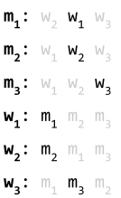
Let’s demonstrate this with an example. We have four agents, and four items:
RSD returns the following lottery (random assignment):
However, every agent prefers the lottery returned by PS:
The PS lottery stochastically dominates the RSD lottery! Since PS returns the ordinal efficient random assignment, there is no other lottery that stochastically dominates this one.
Like ex-post, ordinal efficiency only requires ordinal preferences.
Ordinal efficiency is a stronger property than ex-post. Ordinal efficiency is a weaker property than ex-ante. Ex-ante implies ordinal efficiency. Ordinal efficiency implies ex-post.
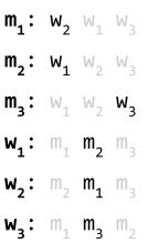
Here’s an example to show that ordinal efficiency is weaker than ex-ante:
PS returns the following lottery for this setting:
Now, in terms of purely ordinal preferences, this is efficient. But what if we got more specific and added cardinal preferences compatible with our ordinal ones?
According to these cardinal preferences, everyone’s expected utilities for the above lottery are (0.6, 0.4, 0.4). However, I can make a new lottery with higher expected utilities:
With this new lottery, everyone’s expected utilities are (0.8, 0.5, 0.5). Higher than our ‘ordinally efficient’ lottery from before! |
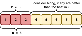
applicants.
How do we maximise our chances of hiring the best secretary? 🤔
candidates. Remember how good they were.
candidates we rejected.
candidates, then just accept the last one.
should we pick?
maximises the chance of us hiring the best
candidate?
(where  , obviously).
 is the event that we accept the best candidate, which
is .
is the best candidate, and we end up picking them.
is the event that we accept the best candidate, which
is .
is the best candidate, and we end up picking them.

 is the event that we accept the best candidate.
was the best candidate, and we pick them or
is the event that we accept the best candidate.
was the best candidate, and we pick them or
 was the best candidate, and we pick them or
 was the best candidate, and we pick them or
 was the best candidate, and we pick them

 .
depends on
.
depends on  . We’re going to have to calculate that first.


 .
.
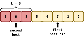
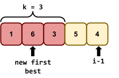
can be reduced to sub-problems:

 , and is the best, then nothing can be better between and
  .
, then we have no choice but to pick when we get to them, because nothing we’ll find
along the way to is gonna be better than anything we found in .
.
, then we have no choice but to pick when we get to them, because nothing we’ll find
along the way to is gonna be better than anything we found in .
Each value is like that applicant’s ‘utility’.
 is just , so:
 , because if everyone has a uniform distribution of
“utility”, everyone has an equal chance of being
‘the best’.
, because if everyone has a uniform distribution of
“utility”, everyone has an equal chance of being
‘the best’.
?
applicants to just :
into  .
th candidate is the best in the subproblem.
.
th candidate is the best in the subproblem.

 .
.


 .
!
.
!
|
|
|
|
|
|
|
|
|
|
|
|

gets closer and closer to our approximated formula
for as tends towards infinity.
that maximises .
 is the optimal value of to maximise .
, the probability tends to
is the optimal value of to maximise .
, the probability tends to  .
.
approaches infinity.
must be really big for those approximations to be
accurate!
? Can we easily find for those situations?
 (I believe) solution that you could use.
, calculate for each, and pick out the with the highest .
(I believe) solution that you could use.
, calculate for each, and pick out the with the highest .
 .
.
 :
:


 yields the highest , so the optimal is 2.
because we’re iterating through all possible
values of , and the number of possible values is
yields the highest , so the optimal is 2.
because we’re iterating through all possible
values of , and the number of possible values is  , and in each of those iterations, we’re calculating , which involves summing fractions from to .
, but is a bit more involved with the maths.
 . Oof!
 . Ooh!
|
Shameless plug: Use DuckDuckGo! 🦆 |
|
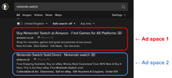
For these examples, I’m going to use DuckDuckGo instead of Google because:
They still sell ad space, but nothing is personalised.
|
slots to sell
Sorry, Xbox players! Maybe in the next example?
 thing.
prices each win a slot.
|
Agent |
Bid |
Allocation |
Payment |
|
1 |
£5 |
First slot |
£4 |
|
2 |
£4 |
Second slot |
£1 |
|
3 |
£1 |
N/A |
N/A |
A small example of GSP, selling two ad slots, with the
setting in yellow and the mechanism result in green.
has a quality score  based on:
 gets the first slot, the second highest bidder
  gets the second slot, etc.


 is the smallest weighted bid that our highest bidding
advertiser could have bidded while still winning the first
ad slot.
’s expected utility =
is the smallest weighted bid that our highest bidding
advertiser could have bidded while still winning the first
ad slot.
’s expected utility = 

|
|
Quality score |
Bid (and true valuation) |
Weighted bid |
Allocation |
Payment |
Utility |
|
Amazon |
0.6 |
£10 |
£6 |
2 |
£3.33 |
4 |
|
eBay |
0.9 |
£7 |
£6.30 |
1 |
£6.67 |
0.3 |
|
CEX |
0.4 |
£5 |
£2 |
N/A |
£0 |
0 |
 is the probability that a user will click on the
ith slot when it is showing the jth advert.
is the probability that a user will click on the
ith slot when it is showing the jth advert.
 (higher-position slots are more likely to be clicked).
 , where:
 is the quality of slot and
 is the quality of bidder .
follows the Power Law.
depends on whether or not the previous ad  was clicked.
prices each win a slot.
was clicked.
prices each win a slot.
|
Allocation |
Agent |
True valuation |
Bid |
Payment |
Utility |
|
1 |
Red |
£5 |
£5 |
£4 |
|
|
2 |
Blue |
£4 |
£4 |
£1 |
|
|
N/A |
Green |
£1 |
£1 |
£0 |
0 |
|
Allocation |
Agent |
True valuation |
Bid |
Payment |
Utility |
|
1 |
Blue |
£4 |
£4 |
£2 |
|
|
2 |
Red |
£5 |
£2 |
£1 |
|
|
N/A |
Green |
£1 |
£1 |
£0 |
0 |
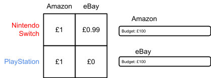
 where, for any bidder :
 for any
 for any
|
Target agent |
Old allocation |
New allocation |
Change in utility |
|
Red |
2 |
1 |
|
|
Red |
2 |
0 |
|
|
Blue |
1 |
2 |
|
|
Blue |
1 |
0 |
|
|
Green |
0 |
2 |
|
|
Green |
0 |
1 |
|
:

|
Allocation |
Agent |
True valuation |
Bid |
Payment |
Utility |
|
1 |
Blue |
£4 |
£4 |
£2 |
|
|
2 |
Red |
£5 |
£2 |
£1 |
|
|
N/A |
Green |
£1 |
£1 |
£0 |
0 |
A copy of the table above
|
Bottom advertiser |
Top advertiser |
Change in utility |
||||||||||||||||||||||||||||
|
Red |
Blue |
|
||||||||||||||||||||||||||||
|
Green |
Red |
|
|
Allocation |
Agent |
True valuation |
Bid |
Payment |
Utility |
|
1 |
Red |
£5 |
£5 |
£2.50 |
|
|
2 |
Blue |
£4 |
£2.50 |
£1 |
|
|
N/A |
Green |
£1 |
£1 |
£0 |
0 |
|
Bottom advertiser |
Top advertiser |
Change in utility |
||||||||||||||||||||||||||||
|
Blue |
Red |
|
||||||||||||||||||||||||||||
|
Green |
Blue |
|
This is why we can’t just tell the truth
when we want to buy ad space.
|
Theorem May’s Theorem (Kenneth May 1952) |
|
Among all possible two-candidate voting systems that never result in a tie, majority rule is the only one that is:
|
|
|
||||||||||||||||||||||||||||||||||||||||||||||||||
|
A vs B |
A vs C |
B vs C |
||||||||||||||||||||||||||||||||||||||||||||||||
|
Winner: A |
Winner: A |
Winner: B |
||||||||||||||||||||||||||||||||||||||||||||||||
|
|
||||||||||||||||||||||||||||||||||||||||||||||||||
|
A vs B |
A vs C |
B vs C |
||||||||||||||||||||||||||||||||||||||||||||||||
|
Winner: A |
Winner: C |
Winner: B |
||||||||||||||||||||||||||||||||||||||||||||||||
|
|
Voter 1 |
Voter 2 |
Voter 3 |
|
1st |
A |
B |
C |
|
2nd |
B |
A |
A |
|
3rd |
C |
C |
B |
candidates.
points.
points, and so on.
|
A: 2+2+2+0+0=6 B: 1+1+1+2+2=7 C: 0+0+0+1+1=2
B is the winner! |
||||||||||||||||||||||||||
|
A: 2+2+2+0+0=6 B: 1+1+1+1+1=5 C: 0+0+0+2+2=4
A is the winner! |
||||||||||||||||||||||||||
No 🤦♂️ not that kind of hare
|
Voting System |
Cons |
|
Condorcet’s Method |
Voting cycle |
|
Plurality Voting |
Fails to satisfy the Condorcet Criterion, manipulable |
|
Borda Count |
Fails to satisfy the Independence of Irrelevant Alternatives (IIA) property |
|
Sequential Pairwise Voting |
Fails to satisfy Pareto efficiency (unanimity) |
|
Hare System |
Fails to satisfy monotonicity |
|
Approval Voting |
Manipulable |
|
Arrow’s Impossibility Theorem |
|
With three or more candidates and any number of voters, there does not exist - and there will never exist - a voting system that satisfies:
|
|
Theorem Arrow’s Impossibility Theorem |
|
When you have three or more candidates, you can’t have a voting system that is:
|
|
Theorem Gibbard-Satterthwaite, 1971 |
|
Every non-dictatorial aggregation rule with >=3 candidates is manipulable. |