Advanced Databases Part 3
Matthew Barnes
Emilia Szynkowska
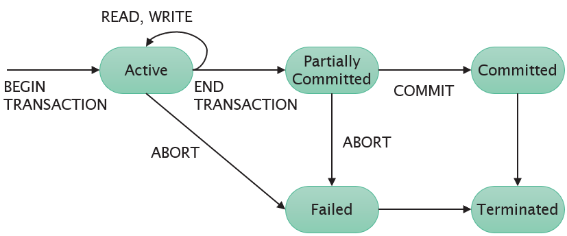
Transactions and Concurrency 2
Granularity and Concurrency 12
Save Points in Transactions 14
Distributed DBMS Principles 36
Implementation of IR Systems 58
|
T1 |
T2 |
XT1 |
YT1 |
XT2 |
YT2 |
Xd |
Yd |
|
read(X) |
|
20 |
|
|
|
20 |
50 |
|
X := X - 10 |
|
10 |
|
|
|
20 |
50 |
|
|
read(X) |
10 |
|
20 |
|
20 |
50 |
|
|
X := X + 5 |
10 |
|
25 |
|
20 |
50 |
|
write(X) |
|
10 |
|
25 |
|
10 |
50 |
|
read(Y) |
|
10 |
50 |
25 |
|
10 |
50 |
|
|
write(X) |
10 |
50 |
25 |
|
25 |
50 |
|
Y := Y + 10 |
|
10 |
60 |
25 |
|
25 |
50 |
|
write(Y) |
|
10 |
60 |
25 |
|
25 |
60 |
|
T1 |
T2 |
XT1 |
YT1 |
XT2 |
YT2 |
Xd |
Yd |
|
read(X) |
|
20 |
|
|
|
20 |
50 |
|
X := X - 10 |
|
10 |
|
|
|
20 |
50 |
|
write(X) |
|
10 |
|
|
|
10 |
50 |
|
|
read(X) |
10 |
|
10 |
|
10 |
50 |
|
|
X := X + 5 |
10 |
|
15 |
|
10 |
50 |
|
|
write(X) |
10 |
|
15 |
|
15 |
50 |
|
read(Y) |
|
10 |
50 |
15 |
|
15 |
50 |
|
CRASH :O |
|
|
|
|
|
|
|
|
rollback |
|
|
|
|
|
20 |
50 |
|
T1 |
T2 |
XT1 |
YT1 |
S |
XT2 |
YT2 |
Xd |
Yd |
|
S := 0 |
|
|
|
0 |
|
|
20 |
50 |
|
|
read(X) |
|
|
0 |
20 |
|
20 |
50 |
|
|
X := X - 10 |
|
|
0 |
10 |
|
20 |
50 |
|
|
write(X) |
|
|
0 |
10 |
|
10 |
50 |
|
read(X) |
|
10 |
|
0 |
10 |
|
10 |
50 |
|
S := S + X |
|
10 |
|
10 |
10 |
|
10 |
50 |
|
read(Y) |
|
10 |
50 |
10 |
10 |
|
10 |
50 |
|
S := S + Y |
|
10 |
50 |
60 |
10 |
|
10 |
50 |
|
|
read(Y) |
10 |
50 |
60 |
10 |
50 |
10 |
50 |
|
|
Y := Y + 10 |
10 |
50 |
60 |
10 |
60 |
10 |
50 |
|
|
write(Y) |
10 |
50 |
60 |
10 |
60 |
10 |
60 |
|
T1 |
T2 |
XT1 |
YT1 |
XT2 |
YT2 |
Xd |
Yd |
|
read(X) |
|
20 |
|
|
|
20 |
50 |
|
|
read(X) |
20 |
|
20 |
|
20 |
50 |
|
|
X := X - 10 |
20 |
|
10 |
|
20 |
50 |
|
|
write(X) |
20 |
|
10 |
|
10 |
50 |
|
read(X) |
|
10 |
|
10 |
|
10 |
50 |
Serial schedule T1 ; T2
|
T1 |
T2 |
XT1 |
YT1 |
XT2 |
YT2 |
Xd |
Yd |
|
read(X) |
|
20 |
|
|
|
20 |
50 |
|
X := X - 10 |
|
10 |
|
|
|
20 |
50 |
|
write(X) |
|
10 |
|
|
|
10 |
50 |
|
read(Y) |
|
10 |
50 |
|
|
10 |
50 |
|
Y := Y + 10 |
|
10 |
60 |
|
|
10 |
50 |
|
write(Y) |
|
10 |
60 |
|
|
10 |
60 |
|
|
read(X) |
10 |
60 |
10 |
|
10 |
60 |
|
|
X := X + 5 |
10 |
60 |
15 |
|
10 |
60 |
|
|
write(X) |
10 |
60 |
15 |
|
15 |
60 |
Serial schedule T2 ; T1
|
T1 |
T2 |
XT1 |
YT1 |
XT2 |
YT2 |
Xd |
Yd |
|
|
read(X) |
|
|
20 |
|
20 |
50 |
|
|
X := X + 5 |
|
|
25 |
|
20 |
50 |
|
|
write(X) |
|
|
25 |
|
25 |
50 |
|
read(X) |
|
25 |
|
25 |
|
25 |
50 |
|
X := X - 10 |
|
15 |
|
25 |
|
25 |
50 |
|
write(X) |
|
15 |
|
25 |
|
15 |
50 |
|
read(Y) |
|
15 |
50 |
25 |
|
15 |
50 |
|
Y := Y + 10 |
|
15 |
60 |
25 |
|
15 |
50 |
|
write(Y) |
|
15 |
60 |
25 |
|
15 |
60 |
Non-Serial and Non-Serialisable Schedule
|
T1 |
T2 |
XT1 |
YT1 |
XT2 |
YT2 |
Xd |
Yd |
|
read(X) |
|
20 |
|
|
|
20 |
50 |
|
X := X - 10 |
|
10 |
|
|
|
20 |
50 |
|
|
read(X) |
10 |
|
20 |
|
20 |
50 |
|
|
X := X + 5 |
10 |
|
25 |
|
20 |
50 |
|
write(X) |
|
10 |
|
25 |
|
10 |
50 |
|
read(Y) |
|
10 |
50 |
25 |
|
10 |
50 |
|
|
write(X) |
10 |
50 |
25 |
|
25 |
50 |
|
Y := Y + 10 |
|
10 |
60 |
25 |
|
25 |
50 |
|
write(Y) |
|
10 |
60 |
25 |
|
25 |
60 |
Non-Serial but Serialisable Schedule
|
T1 |
T2 |
XT1 |
YT1 |
XT2 |
YT2 |
Xd |
Yd |
|
read(X) |
|
20 |
|
|
|
20 |
50 |
|
X := X - 10 |
|
10 |
|
|
|
20 |
50 |
|
write(X) |
|
10 |
|
|
|
10 |
50 |
|
|
read(X) |
10 |
|
10 |
|
10 |
50 |
|
|
X := X + 5 |
10 |
|
15 |
|
10 |
50 |
|
|
write(X) |
10 |
|
15 |
|
15 |
50 |
|
read(Y) |
|
10 |
50 |
15 |
|
15 |
50 |
|
Y := Y + 10 |
|
10 |
60 |
15 |
|
15 |
50 |
|
write(Y) |
|
10 |
60 |
15 |
|
15 |
60 |
|
|
Lock requested |
||
|
Shared |
Exclusive |
||
|
Lock already held by someone else |
None |
Grant |
Grant |
|
Shared |
Grant |
Wait |
|
|
Exclusive |
Wait |
Wait |
|
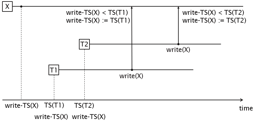
A timestamp TS(T) is a unique identifier used to identify a transaction. The timestamp ordering algorithm orders transactions based on their timestamps. An ordered non-serial schedule should always be serialisable, as the equivalent serial schedule consists of the transactions in order of the timestamp values. The algorithm associates each database item X with two values:
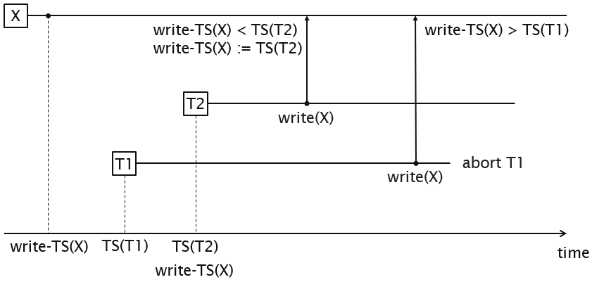
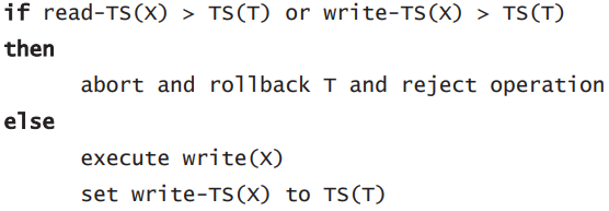
The basic timestamp ordering algorithm compares the timestamps of a transaction T with read_TS(X) and write_TS(X) to ensure the timestamp ordering is valid. If the order is violated, T is aborted and resubmitted to the system with a new timestamp. Any transactions using values edited by T must be rolled back. In cascading rollback, the system keeps rolling back changes as many transactions are dependent on each other.
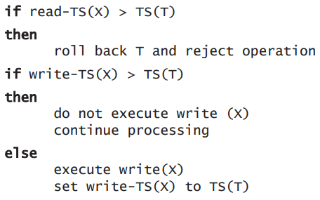
Thomas's write rule is a modification of basic timestamp ordering which does not enforce conflict serialisability and rejects fewer write operations by modifying checks on operations so that obsolete write operations are ignored. If the timestamp of a read operation on an item X is invalid, it is not executed but processing continues. This is because a transaction with a larger timestamp will overwrite the value of X.
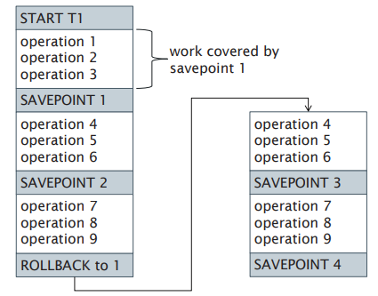
A save point is an identifiable point in a transaction representing a partially consistent state, which can be used to restart a transaction.
A chained transaction is a transaction broken into sub-transactions, which are executed serially.
|
Save Point |
Chained Transaction |
|
allows a transaction to be broken into sub-transactions
database context is preserved
rolls back to an arbitrary save point
does not free unwanted locks |
allows a transaction to be broken into sub-transactions
database context is preserved
rolls back to the previous savepoint
frees unwanted locks |
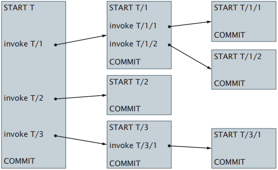
In a nested transaction, a transaction forms a hierarchy of sub-transactions. Here, sub-transactions may abort without aborting their parent transaction. There are three rules for nested transactions:
A saga is a collection of transactions that form a long-duration transaction. A saga is specified as a directed graph where nodes are either actions or terminal nodes abort or complete.
In a saga, each action A has a compensating action A-1. If A is an action and a is a sequence of actions, than AaA-1 ≡ a.
Durability: Once a database is changed and committed, changes should not be lost due to failure
Whenever a transaction is submitted, it will either be committed or aborted. If a transaction fails while executing, any executed operations must be reversed. Failures are classified as transaction, system, or media failures:
To be able to recover from failures that affect transactions, the system maintains a log to store transaction operations and information for recovery. The system log is a sequential, append-only file that is kept on disk so it is not affected by failures. The main memory contains a log buffer, which collects log data and appends it to the log file.
A transaction T reaches its commit point when all its access operations have been executed successfully and the effect of all operations has been recorded in the system log. Beyond the commit point, the effect of the transaction is permanently stored in the database. If a system failure occurs, any transactions which have not been committed are rolled back to undo their effect on the database.
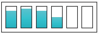
Data that needs to be updated is stored in main memory buffers. It is updated in main memory before being written back to disk. A collection of in-memory buffers called the DBMS cache holds these buffers. When the DBMS requests an item, it first checks the cache to determine whether the item is stored. If not, the item is located on disk and copied into the cache. It may be necessary to flush some of the buffers to make space available for new data.
A log record contains 3 main stages:
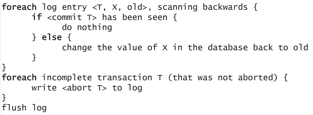
Undo Logging repairs a database following a system crash by undoing the effects of transactions that were incomplete at the time of the crash. Introduces a new record type <T, X, old> showing that T has changed X from its old value.
Rules for Undo Logging:
Recovery with Undo Logging:
In checkpointing, a periodic checkpoint is introduced into the system log. Before a checkpoint, all transactions have either committed or aborted, so that an algorithm will never scan entries before the checkpoint. A new record type <ckpt> is introduced and represents a checkpoint.
Rules for checkpointing:
In nonquiescent checkpointing, we allow transactions to continue during checkpointing. This introduces new record types <start ckpt (T1…Tn)> representing a checkpoint starting with active transactions T1…Tn which have not yet been committed, and <end ckpt>, which represents the end of a checkpoint.
Rules for nonquiescent checkpointing:
Recovery with Checkpointed Undo Logging:
Undo Logging writes <commit T> log records only after all database items have been written to disk. This can potentially cause more disk I/O operations.
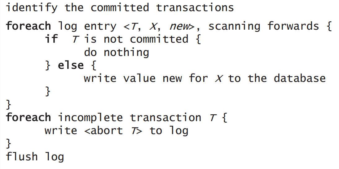
Redo Logging ignores incomplete transactions and repeats changes made by committed transactions to overwrite incorrect values. It writes a <commit T> log record to disk before any values are written to disk, and introduces a new record type <T, X, new> showing that T has changed X to a new value.
Rule for Redo Logging:
Recovery with Redo Logging:
Checkpointing with Redo Logging:
Recovery with Checkpoint Redo Logging:
Undo/Redo Logging aims to address issues with undo and redo logging.
Undo/Redo Logging introduces a new record type <T, X, old new> showing that T has updated X from an old value to a new value.
Rules for Undo/Redo Logging:
Checkpointing with Undo/Redo Logging:
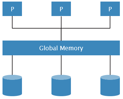
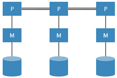
Shared Memory
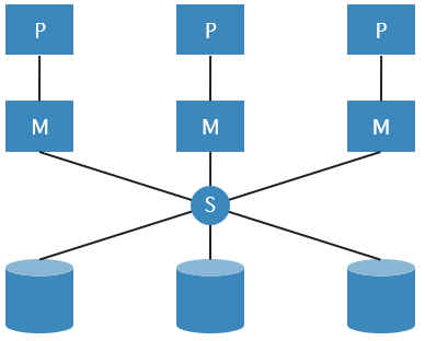
Shared Disc
Shared Nothing
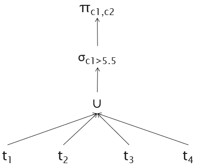
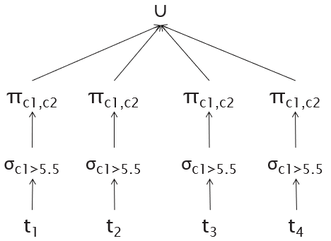
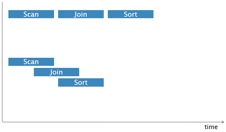
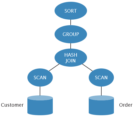
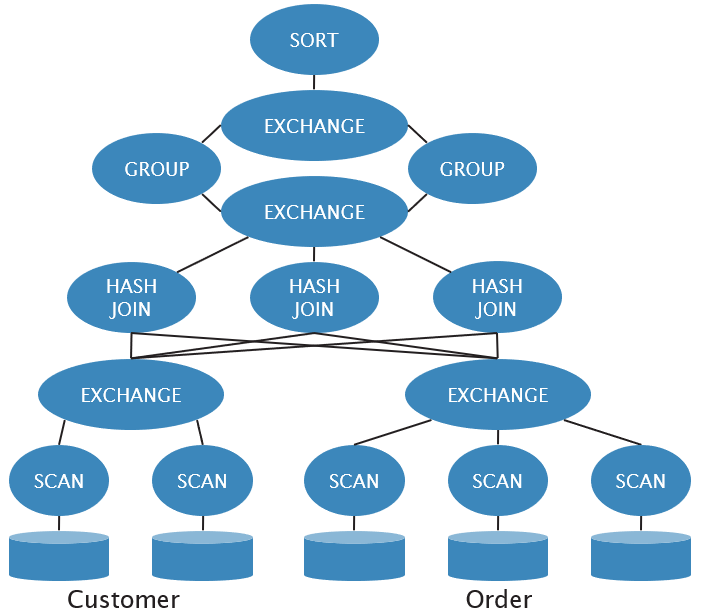
Intra-operator parallelism
Inter-operator parallelism
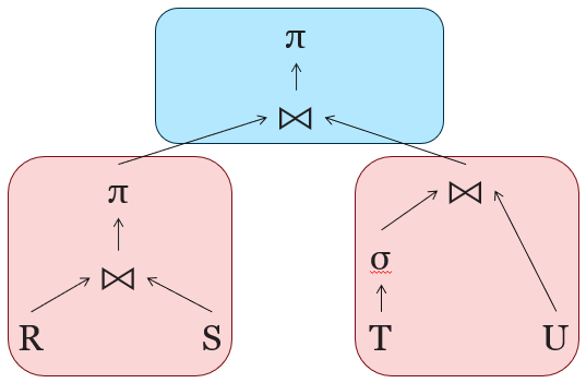
Bushy parallelism
Enquiry
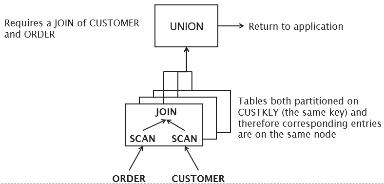
Collocated Join
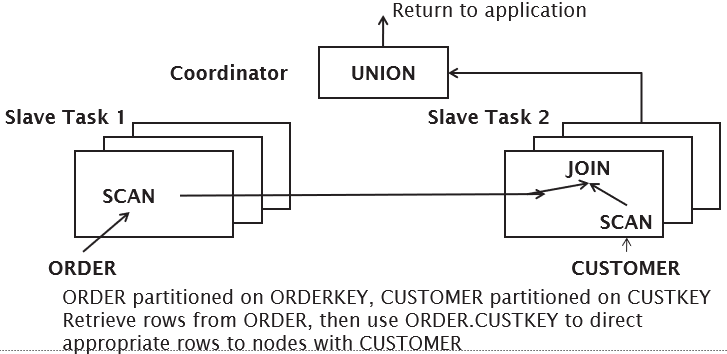
Directed Join
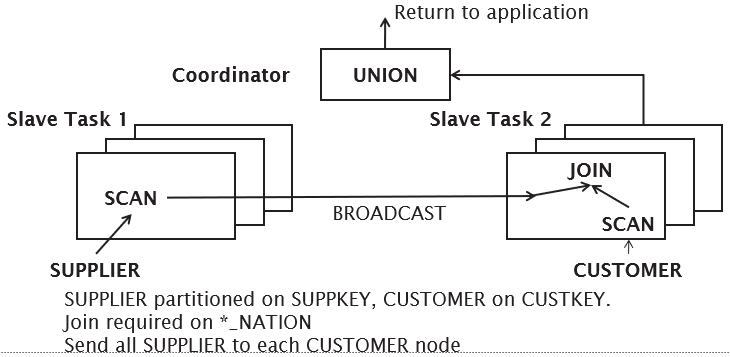
Broadcast Join
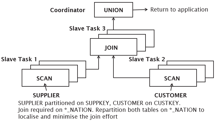
Repartitioned Join
When things go right
|
Principle |
Explanation |
|
Local autonomy |
Each site should be autonomous or independent of each other (low coupling)
Every site should provide their own:
Local operations on a site only affect the local resources of that site, and shouldn’t affect any other site on the network.
This ensures that all the sites are modular, and doesn’t spaghettify the operations of the network. |
|
No reliance on a central site |
The system should not rely on a central site, which may be a single point of failure or bottleneck. |
|
Continuous operation |
The system should never require downtime.
There should be on-line backup and recovery, which are fast enough to be performed online without noticeable performance drops. |
|
Location independence |
Applications shouldn’t even be aware of where the data is physically stored. |
|
Fragmentation independence |
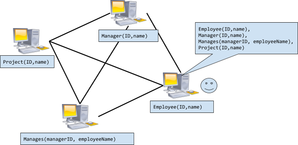
Relations can be divided into fragments and stored at different sites. |
|
Replication independence |
Copies of relations and fragments can be stored on different sites.
This should be under the hood; applications shouldn’t know that duplicates are being maintained and synchronised. |
|
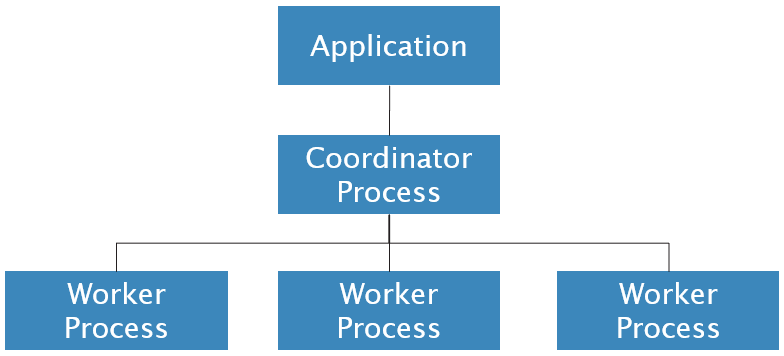
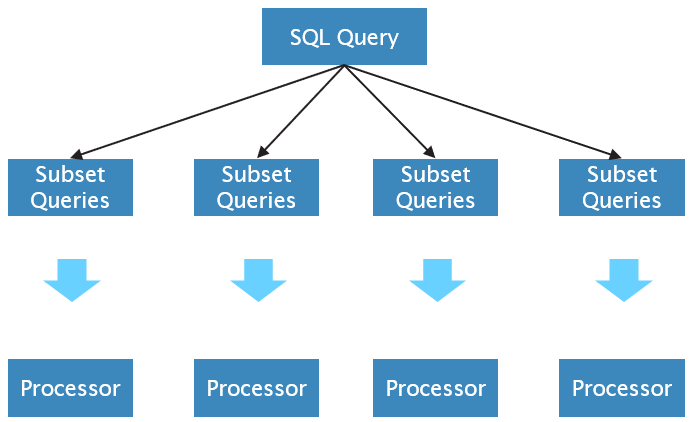
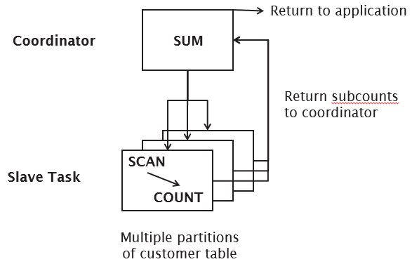
Distributed query processing |
Queries are broken down into component transactions to be executed at the distributed sites (see Parallel Databases for more info). |
|
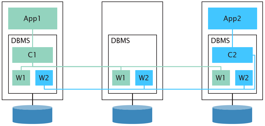
Distributed transaction management |
A system should support atomic transactions (either a transaction happens or it doesn’t). |
|
Hardware independence |
It shouldn’t matter what hardware each site uses; one could be on x86, another could be ARM etc. |
|
Operating system independence |
It shouldn’t matter what OS each site uses; one could be using Linux, another could use Windows etc. |
|
Network independence |
It shouldn’t matter what communication protocols and network topologies are used to connect the sites. |
|
DBMS independence |
It shouldn’t matter what DBMS each site uses; one could be using MySQL, another could use PostgreSQL etc. |

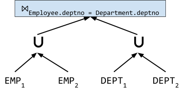
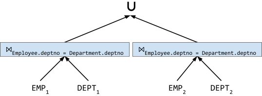
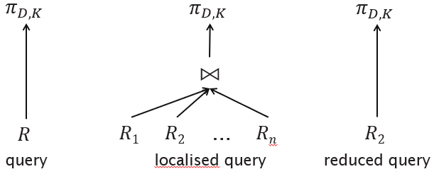
Query
Localised query
Optimised query
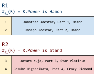
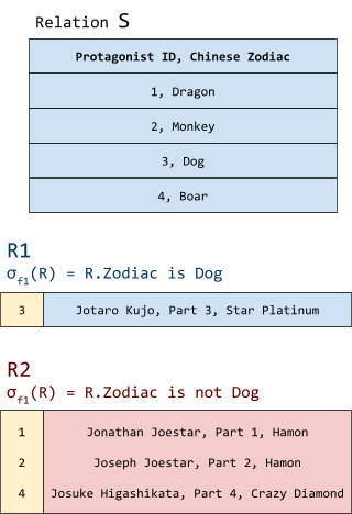
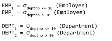
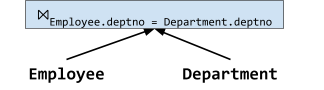
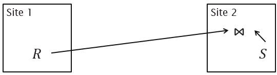
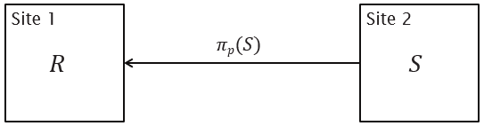
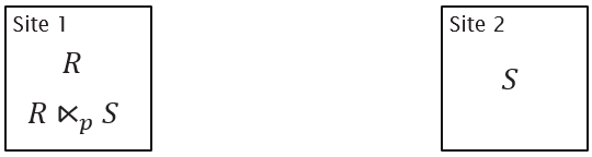
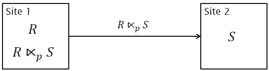
πp(S) projects the attributes used in predicate p over tuples in S
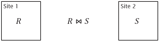
R ⋉p S ≡ πR(R ⨝p πp(S))
R ⨝p S ≡ (R ⋉p S) ⨝p S
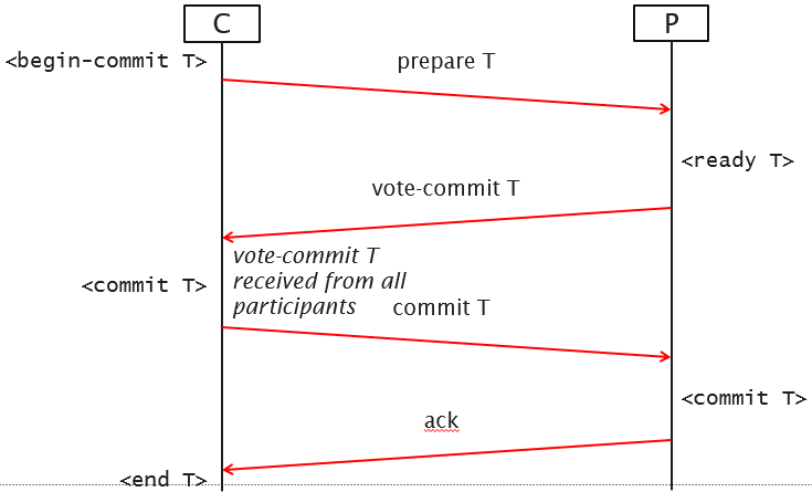
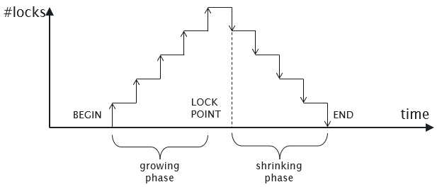
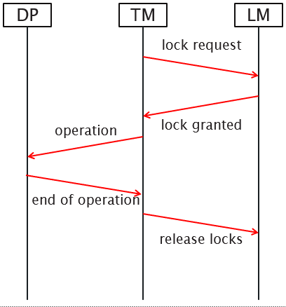
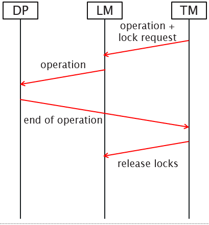
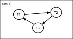
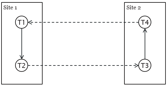
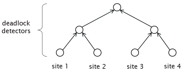
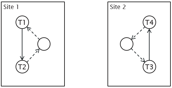
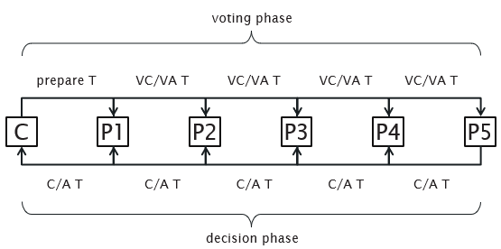
Distributed Two-Phase Locking (2PL)
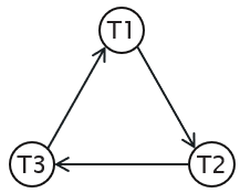
Deadlock
Online Transaction Processing (OLTP) is characterised by a large number of short transactions (INSERT, UPDATE, DELETE) with an emphasis on fast query processing and data integrity.
Online Analytical Processing (OLAP) is characterised by a small number of complex transactions often involving aggregation and multidimensional schemas. Typically, data is taken from a data warehouse. OLAP is ideal for data mining, complex analytical calculations, and business reporting functions such as financial analysis.
Data mining is the process of discovering hidden patterns and relationships in large databases using advanced analytical techniques.
Codd's 12 rules for OLAP:
|
Multidimensional conceptual view |
A multidimensional data model is provided that is intuitively analytical and easy to use. The model decides how users perceive business problems, e.g. time, location, or product. |
|
Transparency |
The technology, underlying data repository, computing architecture and the diverse nature of source data is transparent to users. |
|
Accessibility |
Access is provided only to the data that is needed to perform the specific analysis, presenting a single, coherent and consistent view to the users. |
|
Consistency reporting performance |
Users do not experience any significant reduction in reporting performance as the number of dimensions or the size of the database increases. Users perceive consistent runtime, response time, and machine utilization every time a query is run. |
|
Client-server architecture |
The system conforms to the principles of client-server architecture for optimum performance, flexibility, adaptability and interoperability. |
|
Generic dimensionality |
Every data dimension is logically equivalent in both structure and operational capabilities. |
|
Dynamic sparse matrix handling |
The schema adapts to the specific analytical model being used to optimize sparse matrix handling. |
|
Multi-user support |
Support is provided for users to work concurrently with either the same analytical model or to create different models from the same data. |
|
Unrestricted cross-dimensional operations |
The system recognizes dimensions and automatically performs roll-up and drill-down operations within a dimension or across dimensions. |
|
Intuitive data manipulation |
Consolidation path reorientation, drill-down, roll-up and other manipulations are accomplished intuitively and are enabled directly via point and click actions. |
|
Flexible reporting |
Business users are provided with capabilities to arrange columns, rows and cells in a manner that allows easy manipulation, analysis and synthesis of information. |
|
Unlimited dimensions and aggregation levels |
There can be at least 15 to 20 data dimensions within a common analytical model. |
A data warehouse is a large store of data accumulated from a wide range of sources within a company and used to guide management decisions. A data warehouse is:
Why use a separate data warehouse?
A data warehouse may be stored using:
Data may be accessed using:
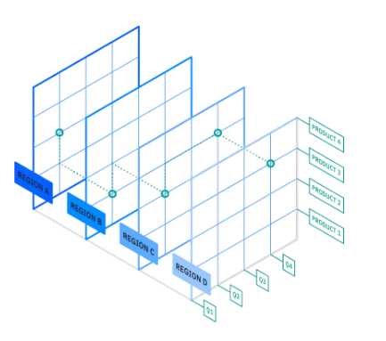
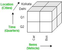
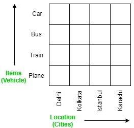
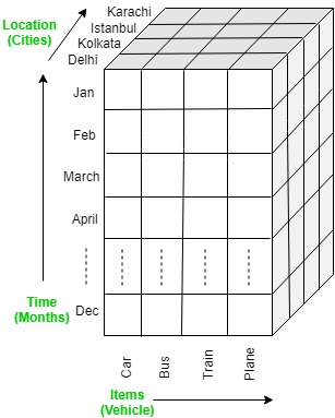
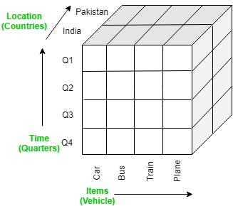
The OLAP cube is an array-based multidimensional database that makes it possible to process and analyse data in multiple dimensions much more efficiently than a traditional relational database. A relational database stored data in a two-dimensional, row-by-column format. The OLAP cube extends this with additional layers, adding additional dimensions to the database. These are often arranged in a hierarchy e.g. country, state, city, store.
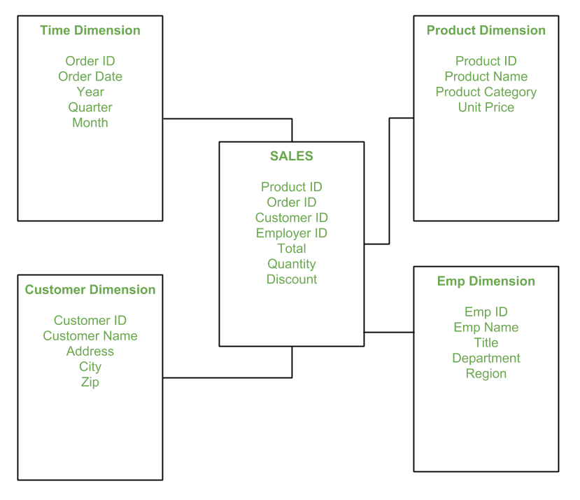
A star schema consists of one fact table connected to a collection of dimension tables. It gets its name from its resemblance to a star shape with the fact table at its center and dimension tables surrounding it.
The primary key of the fact table is a combination of foreign keys from the dimension tables. The rule of referential integrity states that each row in the fact table must contain a primary key value from each dimension table.
Advantages of star schemas:
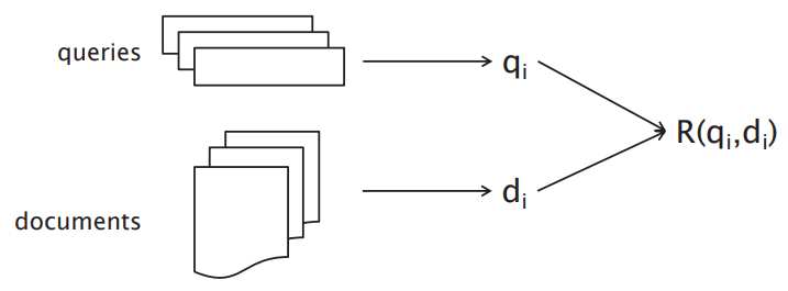
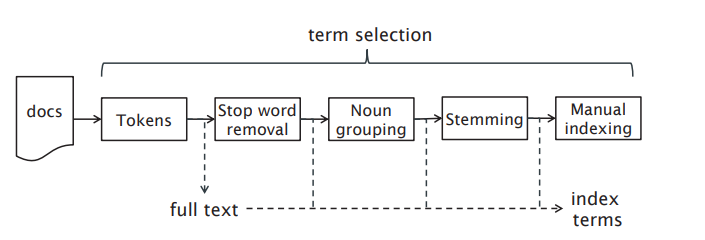
Information Retrieval (IR) is the retrieval of media based on the information a user needs. The user provides a query to the retrieval system, which returns a set of relevant documents from a database. Documents include web pages, scientific papers, news articles, or paragraphs.
An IR model consists of:
IR systems either:
During tokenization, the system identifies distinct words in the document, by separating on whitespace to obtain a list of tokens. It then cleans and prepares the data:
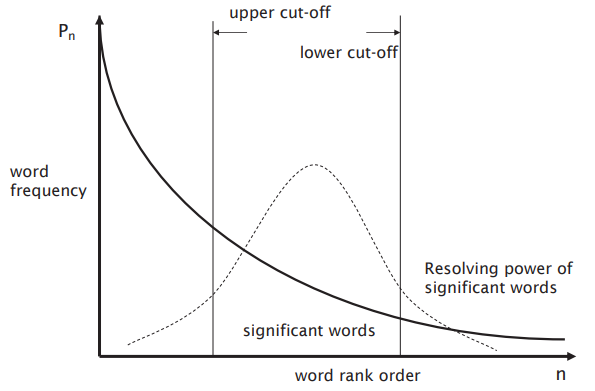
Zipf's law is given by the formula  where na is the rank of a word. This means that the most common words appear
in the middle of the graph, and other words can be ignored. Stopword removal is the process of removing very common words which have
little semantic value such as the, a, at, and, also.
where na is the rank of a word. This means that the most common words appear
in the middle of the graph, and other words can be ignored. Stopword removal is the process of removing very common words which have
little semantic value such as the, a, at, and, also.
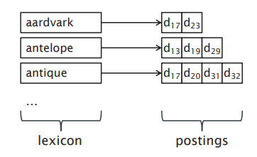
The lexicon is a data structure listing all terms that appear in a collection of documents. This is typically implemented as a hash table for fast lookup. The inverted index is a data structure that contains information about terms in the lexicon. This may include information such as the number of occurrences within documents and pointers to its occurrences (postings).
To calculate the rank of each term:
The boolean model involves querying terms in the lexicon and inverted index, and applying boolean set operators to posting lists to identify relevant documents:
Given the document collection:
d1 = “Three quarks for Master Mark”
d2 = “The strange history of quark cheese”
d3 = “Strange quark plasmas”
d4 = “Strange Quark XPress problem”
The lexicon and inverted index:
three → {d1}
quark → {d1, d2, d3, d4}
master → {d1}
mark → {d1}
strange → {d2, d3, d4}
history → {d2}
cheese → {d2}
plasma → {d3}
express → {d4}
problem → {d4}
The query:
strange AND quark AND NOT cheese
The result set is:
{d2, d3, d4} ∩ {d1, d2, d3, d4} ∩ {d1, d3, d4}
= {d3, d4}
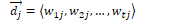
The binary vector model represents documents and queries as vectors of term-based features containing terms t, documents j, and queries q.
Features are binary:
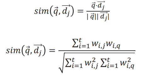
To measure the similarity between a document  and query
  , we can use cosine similarity to produce a binary value. The dot product
  is normalised by the magnitude of each vector.
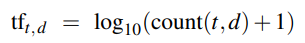
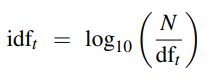
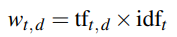
TF-IDF (Term Frequency-Inverse Document Frequency) evaluates the relevance of a term to a document.
Typical queries are ambiguous and can be refined to provide better search results.
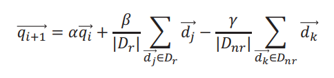
The Rocchio method implements query refinement through relevance feedback. The query is first executed to provide the user with initial
results. The user tags each result as relevant or non-relevant,
allowing the model to adjust its weights. The improved query  is created using the new weights and the user adjusts this
until the results are satisfactory. Typical starting weights are
α = 1, β = 0.75,
is created using the new weights and the user adjusts this
until the results are satisfactory. Typical starting weights are
α = 1, β = 0.75,  = 0.25. (nope, I don’t understand this formula either)
Relevance is the key to determining the effectiveness of an IR system. Precision and recall are two common statistics used to determine the effectiveness of a system. F1 combines precision and recall by taking the harmonic mean between them.
TP (True Positive): "yes" data is correctly predicted as "yes"
TN (True Negative): "no" data is correctly predicted as "no"
FP (False Positive): "no" data is incorrectly predicted as "yes"
FN (False Negative): "yes" data in incorrectly predicted as "no"
Accuracy = 
proportion of correct predictions
Precision = 
proportion of correct positive predictions out of all positive predictions
i.e. how many positive predictions were correct?
Recall = 
proportion of correct positive predictions out of all correct predictions
i.e. how many correct predictions were made?
F1 =  or
or 
harmonic mean of precision and recall
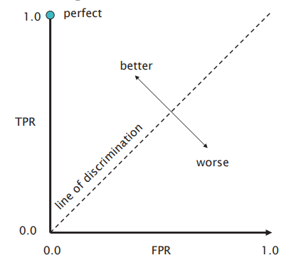
ROC Curve (Receiver Operating Characteristic): plots true positive rate (recall) against false positive rate

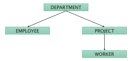
The first hierarchical database was the IBM Information Management System, developed in 1966 to support the Apollo programme. Hierarchical databases are built as trees of related record types connected by parent-child relationships.
An occurence of a parent-child relationship (PCR) consists of:
A database may contain many hierarchical occurrence trees:
Disadvantages of hierarchical databases:
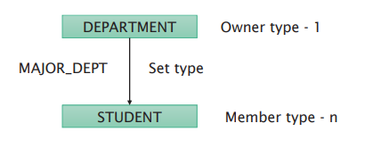
Network databases were standardised by the Conference on Data Systems Languages committee in 1969. A network database allows 1:N (one-to-many) relationships between records and files.
An occurrence of a set consists of:
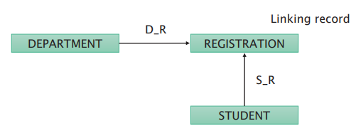
Set types can only represent one-to-many relationships. To create many-to-many relationships, a dummy record can be used to join two record types.
Advantages of network databases:
Disadvantages of network databases:
A native XML database allows data to be specified and stored in XML format.
Object-relational impedance mismatch is a set of conceptual and technical difficulties that are often encountered when a relational database is being served by an application program written in an object-oriented language, as objects and classes must be mapped to database tables defined by the relational schema. Impedance mismatch can be addressed by using a NoSQL database.
NoSQL is an approach to database design that provides flexible schemas for the storage and retrieval of data beyond the traditional table structures found in relational databases. NoSQL databases are:
NoSQL data types: