Advanced Databases Part 1
Matthew Barnes
Multidimensional Access Structures 71
|
Part 1 |
|
✅ Data types |
|
✅ DBMS Architecture |
|
✅ Data Storage |
|
✅ Access Structures |
|
✅ Multidimensional Access Structures |
|
✅ Relational Algebra |
|
✅ Problems and Complexity in Databases |
|
✅ Conjunctive Queries - Containment and Minimisation |
|
✅ Query Processing |
|
✅ Data Integration |
|
✅ Ontology Based Data Integration |
|
✅ Transactions and Concurrency |
|
✅ Advanced Transactions |
|
✅ Logging and Recovery |
|
✅ Parallel Databases |
|
✅ Distributed Databases |
|
✅ Data Warehousing |
|
✅ Information Retrieval |
|
✅ Non-Relational Databases |
|
Stream Processing (not examined) |
|
Peer to Peer Systems (not examined) |
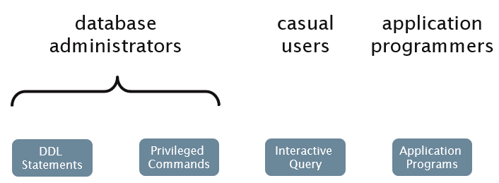
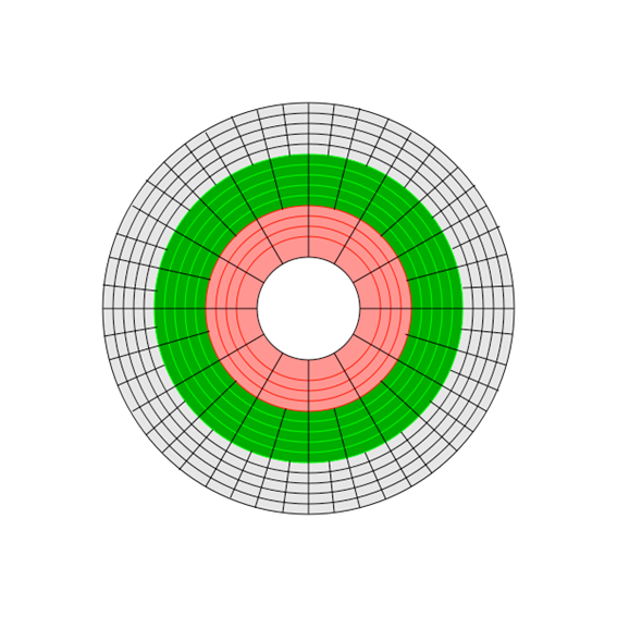
DBMS Interfaces (what is exposed to us)
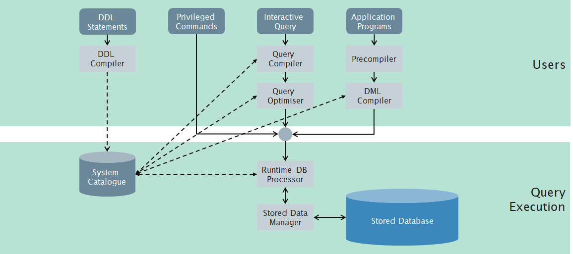
DBMS Components (how it all works)
|
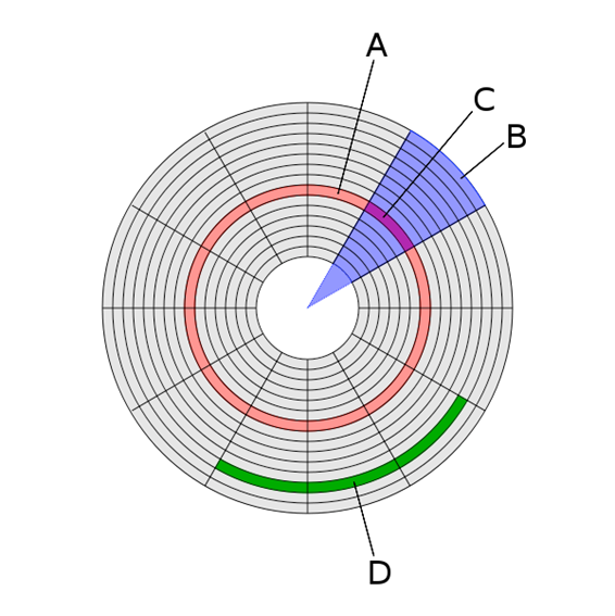
gap |
sync |
mark |
data |
ecc |
|
Rotational speed (rpm) |
Average delay (ms) |
|
4,200 |
7.14 |
|
5,400 |
5.56 |
|
7,200 |
4.17 |
|
10,000 |
3.00 |
|
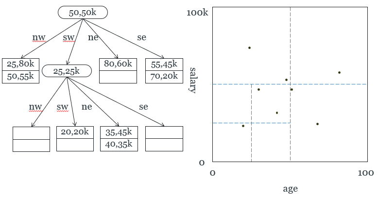
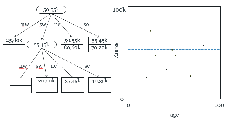
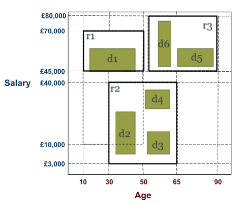
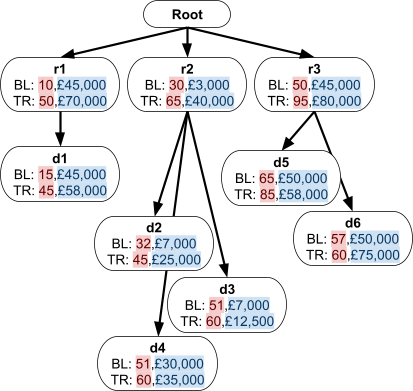
15,000 |
2.00 |
|
|
HDD |
SDD |
|
Random Read IOPS |
125-150 IOPS |
~50,000 IOPS |
|
Random Write IOPS |
125-150 IOPS |
~40,000 IOPS |


|
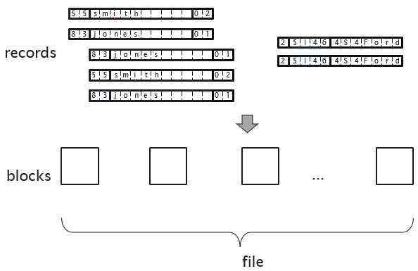
5 |
5 |
s |
m |
i |
t |
h |
|
|
|
|
|
0 |
2 |
|
8 |
3 |
j |
o |
n |
e |
s |
|
|
|
|
|
0 |
1 |
|
{ |
|
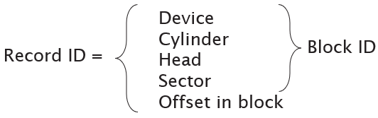
Logical ID |
Physical ID |
|
56 |
5AF8 |
|
57 |
|
|
58 |
2DE0 |
|
A block of memory |
||||||
|
Logical ID |
|
56 |
|
|
|
|
|
Physical ID |
5AF0 |
5AF8 |
5B00 |
5B08 |
5B10 |
5B18 |
|
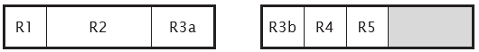
Data |
5B |
|
3F |
02 |
7A |
|
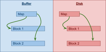
5B00 and above can be reused, but 5AF8 can never be reused.
|
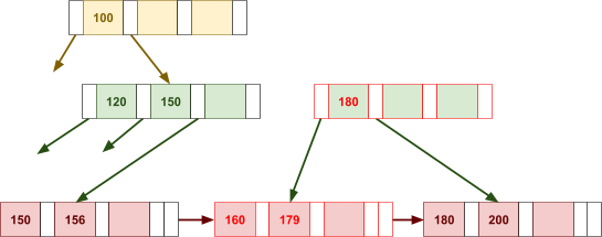
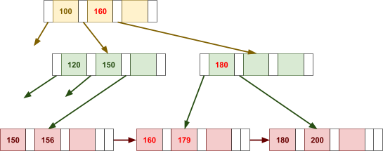
Before |
After |
|
|
|
|
Before |
After |
|
|
|
|
Before |
After |
|
|
|
|
Before |
After |
|
|
|
|
Before |
After |
|
|
|
|
Before |
After |
|
|
|
|
Before |
After |
|
|
|
|
Before |
After |
|
|
|
|
Hash so far |
Operation + Explanation |
|
|
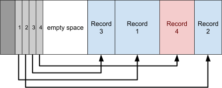
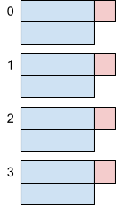
Nothing
We haven’t done anything so far.
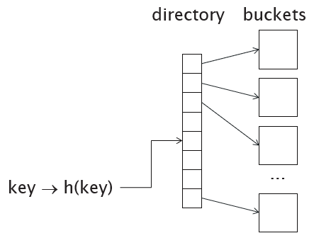
Ah alright; if you really want to be pedantic about it, we’ve initialised our hash table with 4 buckets, containing 2 records per bucket. |
|
|
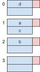
Insert a, b, c, d
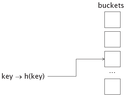
h(a) = 1 h(b) = 2 h(c) = 1 h(d) = 0
For each key, we hash it using the values above and we “append” that key (or record) to the associated bucket.
For example, when we hash ‘a’ into ‘1’, we look up the bucket labelled ‘1’ and insert our key ‘a’ there. |
|
|
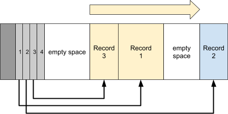
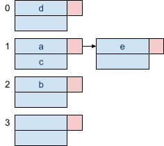
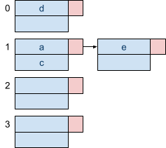
Insert e
h(e) = 1
Like above, we try to insert ‘e’ into bucket ‘1’ according to the hash function.
However, bucket ‘1’ is full, therefore we add an overflow bucket to extend the capacity of bucket ‘1’. We then put ‘e’ into that overflow bucket. |
|
|
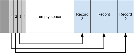
Delete b
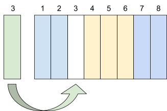
When we delete a key, we can just remove it from the bucket. If there were any keys after it, we can just move them up the bucket. |
|
|
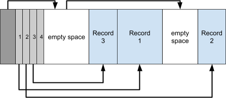
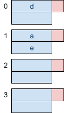
Delete c
By deleting ‘c’, we’re freeing space for ‘e’ in the bucket it’s leading from, so we can move ‘e’ from the overflow bucket to the original bucket and remove the overflow bucket. |
|
Hash so far + Operation |
Operation + Explanation |
|
|
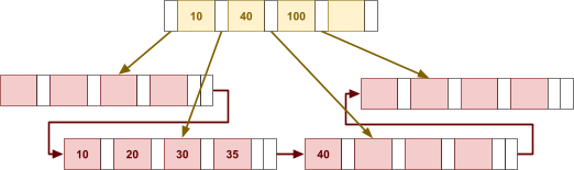
Nothing
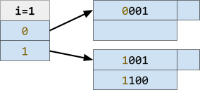
The variable i is just 1, and we have three keys. |
|
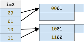
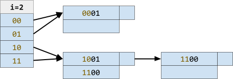
Increase i to 2
Partition “10” and “11” into different buckets
Add “1010” to the “10” bucket
|
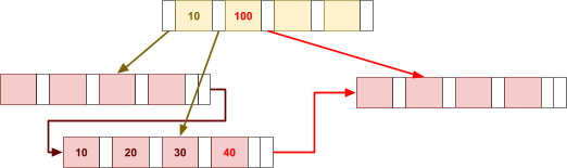
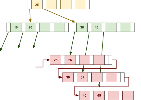
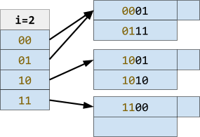
Insert 1010
To insert 1010, we could just put 1010 into the ‘1’ directory. However, that directory is full.
Therefore we need to increase i from 1 to 2.
Then we partition “10” and “11” into different buckets, leaving us with enough space to put “1010” into the “10” bucket.
|
|
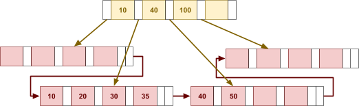
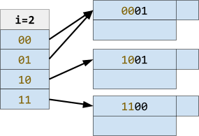
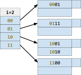
Add “0111” to the “01” bucket
|
Insert 0111
Since the “01” bucket has enough space for one more key, we can place “0111” into the “01” bucket.
It just so happens that “00” and “01” share the same bucket. However, if we need to add one more key they’ll need their own buckets. |
|
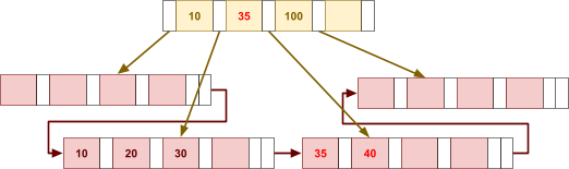
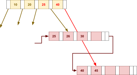
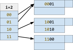
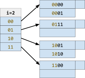
Partition “00” and “01” into different buckets
Add “0000” to the “00” bucket
|
Insert 0000
Speak of the devil! There isn’t enough space in the “00” bucket, so we’ll need to split “00” and “01” into their own buckets.
Then we’ll have enough space to put 0000 into the “00” bucket. |
|
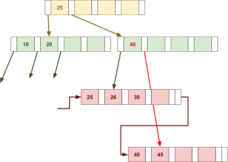
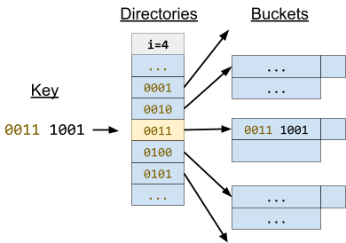
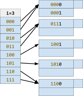
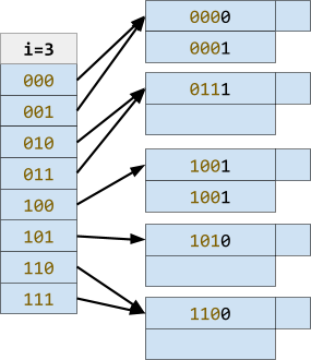
Increase i to 3
Partitioning “100” and “101” into different blocks
Add “1001” to the “100” bucket
|
Insert 1001
Don’t worry, this is the last operation!
If we look at bucket “10”, we’ll see it’s full again.
Like last time, we need to increment i to 3.
“100” and “101” will then share a bucket. We will split that into two, so “100” and “101” will have their own buckets.
We will then have enough space in bucket “100” to put 1001 in.
Duplicate keys are allowed, in case you were wondering. |
|
Hash so far + Operation |
Operation + Explanation |
|
|
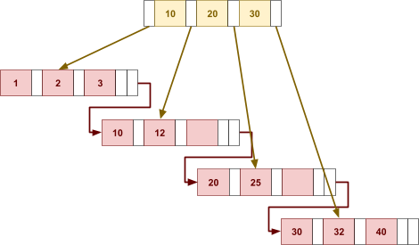
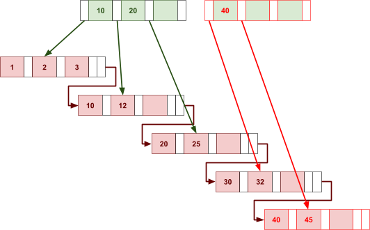
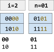
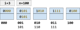
Nothing
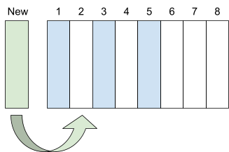
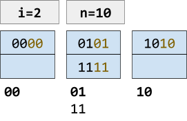
Here we have a linear hash where i = 2, and the maximum value bucket we have is 01 (n).
The bold numbers underneath the blue buckets are the bucket values.
If we find a value of m equal to a bucket value or a number underneath a bucket value, the key will be added to that bucket.
As you can see on the left, for example, 11 is underneath bucket value 01, so 0101 will redirect to bucket 01, and 1111 will be redirected to bucket 01 (see the case for n ≤ m < 2i above)
In a way, the pairs 00, 10 and 01, 11 “share” buckets, a bit like how extensible hashing shared buckets. |
|
|
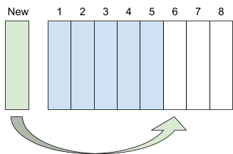
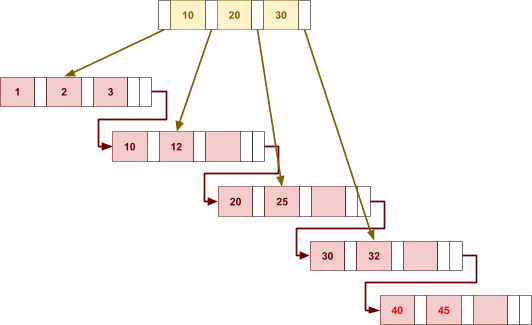
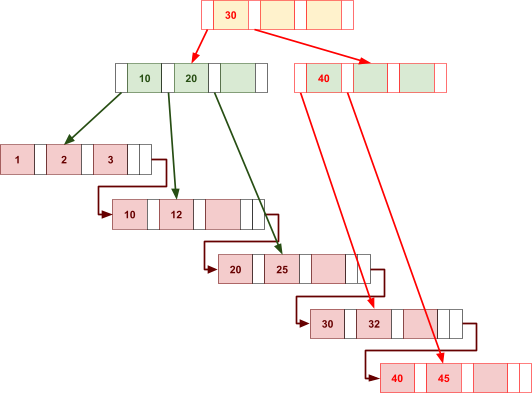
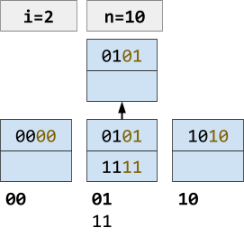
Increment n
If our buckets get too crowded, we can add a new bucket. This is similar to that partitioning / splitting thing we did with extensible hashing.
Here we give “10” its own bucket, so now we can move all the keys where m = 10 over to the new 10 bucket. |
|
|
Insert 0101
If the key K = 0101 and i = 2, then m = 01. This should go into bucket 01.
Since it’s full, we can use an overflow block. |
|
|
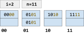
Increment n
If we increment n, we’re giving 11 their own bucket. Therefore we can move the key 1111 to the new bucket 11.
With the new space available in bucket 01, we can move 0101 out of the overflow block and into the main block.
However, now we’ve reached the maximum number of buckets we can create where i = 2. If we want more, we need to increase i. |
|
|
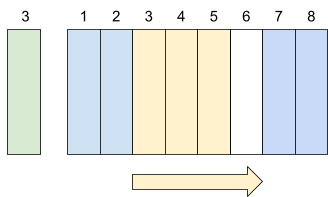
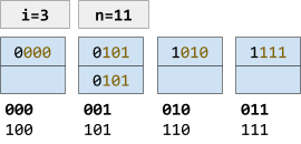
Increment i
Incrementing i doesn’t change the capacity per se, but it changes the potential for capacity increase.
As you can see the buckets are shared again; notice that there are m = 101 keys in the 001 bucket or m = 111 keys in the 011 bucket, for example. |
|
|
Increment n and insert 100
Now, there is space in the 000 bucket, so we could just insert 100 in there, but let’s try to spread out our keys into different buckets more.
When we add the 100 bucket, m = 000 and m = 100 no longer share the same bucket.
Therefore we can now add 100 into its own 100 bucket. |
|
SELECT ... |
|
SELECT ... |